
ROC Curve ve AUC Nedir? Sınıflandırma Modellerini Karşılaştırma
AUC %85 doğruluk demek değildir. ROC eğrisinin iki eksenini elle hesaplamaktan AUC'nin gerçek yorumuna, eşiğin neden ayrı bir iş kararı olduğundan dengesiz veride neden yanıltabileceğine kadar.
- Makine Öğrenmesi
- İstatistik
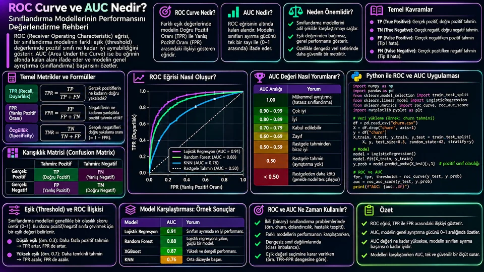
ROC eğrisi neyi gösterir?
İkili bir sınıflandırıcı aslında doğrudan "evet/hayır" üretmez. Her gözlem için pozitif sınıfa ait bir skor ya da olasılık verir. "Evet" kararı, bu skoru bir eşikle karşılaştırdığınızda ortaya çıkar. Eşiği 0,5'ten 0,3'e indirdiğinizde model daha cömert davranır: daha çok gerçek pozitif yakalar ama daha çok yanlış alarm da üretir.
ROC eğrisi (Receiver Operating Characteristic) işte bu değiş tokuşun haritasıdır. Olası her eşik için iki oran hesaplanır ve bir nokta olarak çizilir.
Eşiği çok yüksek tuttuğunuzda neredeyse hiçbir şey pozitif seçilmez; iki oran da sıfıra yaklaşır ve eğri sol alt köşeden başlar. Eşiği en aşağı indirdiğinizde her şey pozitif sayılır; iki oran da 1'e ulaşır ve eğri sağ üst köşede biter. Arasındaki yol, modelin pozitifleri negatiflerden ne kadar iyi sıraladığını gösterir.
Tek bir eşiği elle hesaplayalım
Soyut kalmaması için somut bir örnek: 100 gerçek pozitif ve 900 gerçek negatif gözlemimiz olsun. Belirli bir eşikte model şu sonucu veriyor.
| Model: Pozitif | Model: Negatif | Toplam | |
|---|---|---|---|
| Gerçek: Pozitif | TP = 80 | FN = 20 | 100 |
| Gerçek: Negatif | FP = 90 | TN = 810 | 900 |
Buradan TPR = 80 / 100 = 0,80 ve FPR = 90 / 900 = 0,10 çıkar. Bu eşik, ROC eğrisi üzerinde (0,10 ; 0,80) noktasıdır. Eşiği biraz daha düşürürseniz nokta sağa ve yukarı kayar: daha çok hasta yakalarsınız, daha çok sağlıklı kişiyi boşuna uyarırsınız.
Dikkat edilecek bir nokta: 90 yanlış pozitif, oran olarak sadece %10 görünüyor. Ama mutlak sayı olarak 90 kişi — bu, gerçek bir operasyonda 90 ek telefon, 90 ek inceleme demek. Oranın küçük olması iş yükünün küçük olduğu anlamına gelmez.
AUC ne anlama gelir?
AUC (Area Under the Curve), ROC eğrisinin altında kalan alandır ve tek bir sayıya iner. En kullanışlı yorumu şudur: rastgele seçilmiş bir pozitif örneğin skoru, rastgele seçilmiş bir negatif örneğin skorundan ne sıklıkta yüksektir? Eşit skorlar bu hesapta yarım sayılır.
Yani AUC = 0,85 demek, "model %85 doğru tahmin ediyor" demek değildir. "Rastgele bir pozitif–negatif çiftinde, pozitif olanın skoru %85 olasılıkla daha yüksektir" demektir. Bu ayrım önemli, çünkü AUC bir doğruluk ölçüsü değil, bir sıralama kalitesi ölçüsüdür.
| AUC | Sezgi | Nasıl yorumlanır? |
|---|---|---|
| 0,50 | Yazı tura | Bu veride ayırt edici sinyal yok denecek kadar az. |
| 0,70 | Bir miktar ayrım | Yeterli mi, tamamen kullanım amacına bağlı. |
| 0,85 | Güçlü sıralama | Çoğu eşikte pozitifler negatiflerin üstünde. |
| 0,99+ | Neredeyse kusursuz | Önce veri sızıntısı olup olmadığına bakın. |
Son satırı özellikle vurgulamak istiyorum. Gerçek bir projede 0,99'un üzerinde AUC gördüğünüzde ilk tepkiniz sevinmek değil, şüphelenmek olmalı. Genellikle açıklaması şudur: hedefin bir türevi özellik olarak modele sızmıştır, ya da eğitim ve test kümeleri arasında aynı kayıt tekrarlanmıştır.
Ayrıca bu değerler evrensel kalite etiketi değildir. Tıbbi tarama ile reklam tıklama tahmininde "iyi AUC" aynı sayı değildir; alan, veri kalitesi ve hata maliyeti belirleyicidir.
Python ile ROC ve AUC
Aşağıdaki örnek, scikit-learn'ün meme kanseri veri kümesinde bir lojistik regresyon eğitiyor. Bu veri kümesinde sınıf 1 benign (iyi huylu) etiketine karşılık gelir; pozitif sınıfı açıkça belirtmek, sonradan ters okumaların önüne geçer.
import matplotlib.pyplot as plt
from sklearn.datasets import load_breast_cancer
from sklearn.linear_model import LogisticRegression
from sklearn.metrics import roc_curve, roc_auc_score
from sklearn.model_selection import train_test_split
from sklearn.pipeline import make_pipeline
from sklearn.preprocessing import StandardScaler

data = load_breast_cancer()
X_train, X_test, y_train, y_test = train_test_split(
    data.data, data.target, test_size=0.25,
    stratify=data.target, random_state=42
)

model = make_pipeline(
    StandardScaler(),
    LogisticRegression(max_iter=2000)
).fit(X_train, y_train)

# Sütun 1, model.classes_[1] sınıfına aittir
y_score = model.predict_proba(X_test)[:, 1]

fpr, tpr, thresholds = roc_curve(y_test, y_score, pos_label=1)
auc = roc_auc_score(y_test, y_score)
print(f"AUC: {auc:.3f}")    # AUC: 0.998

plt.plot(fpr, tpr, label=f"Lojistik regresyon (AUC={auc:.3f})")
plt.plot([0, 1], [0, 1], "--", color="gray", label="Rastgele")
plt.xlabel("Yanlış pozitif oranı (FPR)")
plt.ylabel("Doğru pozitif oranı (TPR)")
plt.legend(); plt.grid(alpha=0.25); plt.show()
Bu veri kümesinde AUC yaklaşık 0,998 çıkar. Tam da yukarıda uyardığım bölgede — ama burada açıklaması masum: bu küme ders kitabı örneği olarak seçilmiş, sınıfları gerçekten iyi ayrılan bir veridir. Kendi projenizde aynı sayıyı gördüğünüzde aynı rahatlıkla kabul etmeyin.
predict() çıktısını (0/1 etiketler) değil, predict_proba() veya decision_function() skorunu kullanın. Sadece etiket verirseniz eğri tek bir noktaya çöker ve AUC anlamını yitirir. Ayrıca predict_proba sütunlarının sırası model.classes_ ile belirlenir; pozitif sınıfın hangi sütunda olduğunu doğrulayın.İki modeli karşılaştırmak
Model karşılaştırmasında kural basit ama sık ihlal edilir: aynı test kümesi, aynı pozitif sınıf tanımı, aynı ön işleme. Bunlardan biri değişirse karşılaştırma geçersizdir.
from sklearn.ensemble import RandomForestClassifier

modeller = {
    "Lojistik regresyon": model,
    "Random Forest": RandomForestClassifier(
        n_estimators=300, random_state=42
    ).fit(X_train, y_train),
}

for ad, clf in modeller.items():
    skor = clf.predict_proba(X_test)[:, 1]
    print(f"{ad}: AUC={roc_auc_score(y_test, skor):.3f}")

# Lojistik regresyon: AUC=0.998
# Random Forest:      AUC=0.995
Burada 0,998 ile 0,995 arasındaki fark, 143 gözlemlik tek bir test bölmesinden geliyor. Bu kadar küçük bir farkı "lojistik regresyon daha iyi" diye raporlamak yanıltıcı olur. Küçük veri kümelerinde tek bölme yerine çapraz doğrulama yapıp sonuçların hem ortalamasını hem de değişkenliğini verin.
Bir başka incelik: iki modelin ROC eğrileri kesişebilir. Genel alanı büyük olan model, sizin çalışmayı planladığınız düşük FPR bölgesinde daha kötü olabilir. Eğrileri aynı grafiğe çizin ve ilgilendiğiniz aralığa bakın.
Eşik seçimi ayrı bir karardır
AUC yüksek diye model sahada iyi çalışmaz; eşiği de doğru seçmeniz gerekir. Üstelik bu seçim istatistiksel değil, iş kararıdır: iki hata türünün maliyeti nedir?
| Senaryo | Pahalı olan hata | Eşik yönü |
|---|---|---|
| Hastalık taraması | Hastayı kaçırmak (FN) | Düşür — recall'ü yükselt |
| Spam filtresi | Önemli e-postayı engellemek (FP) | Yükselt — precision'ı koru |
| Dolandırıcılık tespiti | Duruma göre değişir | İnceleme kapasitesine göre ayarla |
| Churn arama listesi | Boşa yapılan arama (FP) | Kapasiteye göre üstten N kişi seç |
Son satır pratikte çok işe yarar. Çağrı merkeziniz günde 200 arama yapabiliyorsa, "eşik kaç olmalı" sorusunun cevabı aslında "skoru en yüksek 200 kişiyi al"dır. Eşik, kapasitenin bir sonucu olur.
Sınıf dengesizliğinde ROC yanıltabilir
ROC'nin FPR paydasında gerçek negatifler vardır. Negatif sınıf çok büyükse bu payda şişer ve FPR olduğundan küçük görünür. Somut bir örnek verelim: 1.000.000 işlemde 1.000 dolandırıcılık var. Modeliniz FPR = 0,01 ile çalışıyor; kulağa harika geliyor. Ama bu, 999.000 temiz işlemin %1'i, yani yaklaşık 9.990 yanlış alarm demek. Gerçek dolandırıcılıkların hepsini yakalasanız bile, inceleme listenizin onda dokuzu boş çıkacak.
Bu yüzden nadir pozitif sınıf durumunda Precision–Recall eğrisi ve Average Precision (AP) daha bilgilendiricidir. PR eğrisi, "pozitif dediklerimin ne kadarı gerçekten pozitifti?" sorusunu doğrudan görünür kılar ve negatif sınıfın büyüklüğünden ROC kadar etkilenmez.
AUC'nin söylemedikleri
Eşik performansı
AUC bütün eşiklerin ortalaması gibidir; sizin kullanacağınız tek eşikte ne olacağını söylemez.
Kalibrasyon
Skorlar iyi sıralanmış olabilir ama "0,8" gerçekten %80 olasılık anlamına gelmeyebilir. Kalibrasyon ayrı ölçülür.
Belirsizlik
Tek bir test örneklemindeki AUC bir tahmindir. 0,91 ile 0,89 arasındaki fark gürültü olabilir.
Alt gruplar
Genel AUC yüksekken belirli bir müşteri segmentinde model çok daha kötü olabilir. Ayrı ayrı bakın.
Veri kayması
Test anındaki dağılım canlıda değişirse AUC de değişir. Üretimde izlemeye devam edin.
Çok sınıflılık
İkiden fazla sınıfta one-vs-rest mi one-vs-one mu, macro mu weighted mi — yöntemi raporda belirtin.
Kalibrasyon konusu özellikle gözden kaçar. Bir skoru doğrudan beklenen değer hesabında kullanacaksanız (örneğin "bu müşterinin ayrılma olasılığı × yaşam boyu değeri"), sıralama yetmez; olasılığın gerçekten olasılık olması gerekir. Bunun için kalibrasyon eğrisi veya Brier skoru kullanın.
Uygulamalı değerlendirme akışı
- Pozitif Sınıfı
Tanımla - Veriyi
Böl - Skorları
Al - ROC ve AUC
Hesapla - Eşiği
Seç - Testte
Raporla
- Pozitif sınıfı iş açısından tanımlayın ve iki hata türünün maliyetini yazın.
- Eğitim, doğrulama ve test bölmelerini ayırın; zaman boyutu varsa kronolojik bölün.
- Olasılık veya karar skorunu alın, etiketleri değil.
- ROC eğrisini çizin, AUC'yi bağımsız veride hesaplayın.
- Eşiği doğrulama verisinde iş hedefine göre seçin.
- Test kümesinde confusion matrix, precision, recall ve mutlak hata sayılarını raporlayın.
Sonuç
ROC eğrisi, bir sınıflandırıcının farklı eşiklerde yakaladığı pozitifler ile ürettiği yanlış alarmlar arasındaki dengeyi gösterir. AUC bu eğriyi tek sayıya indirir ve modelin sıralama kalitesini özetler — doğruluğunu değil.
Pratikte en işe yarayan yaklaşım, AUC'yi bir başlangıç noktası olarak görmektir. Modeli seçerken AUC'ye bakın; sahaya çıkarırken eşiği, mutlak hata sayılarını ve o eşikteki confusion matrix'i konuşun. Sınıf dengesizse PR eğrisini de ekleyin. Tek bir sayı hiçbir zaman kararın tamamı olmamalı.
What does a ROC curve show?
A binary classifier does not really produce "yes/no" directly. For every observation it gives a score or probability for the positive class. The "yes" decision appears only when you compare that score against a threshold. Lower the threshold from 0.5 to 0.3 and the model becomes more generous: it catches more true positives, but it also raises more false alarms.
The ROC (Receiver Operating Characteristic) curve is the map of that trade-off. For every possible threshold, two rates are computed and plotted as a point.
Keep the threshold very high and almost nothing is selected as positive; both rates approach zero and the curve starts in the bottom-left corner. Lower it all the way and everything counts as positive; both rates reach 1 and the curve ends in the top-right corner. The path in between shows how well the model ranks positives above negatives.
Working one threshold out by hand
To keep it concrete: suppose we have 100 true positives and 900 true negatives. At a particular threshold the model produces this.
| Model: Positive | Model: Negative | Total | |
|---|---|---|---|
| Actual: Positive | TP = 80 | FN = 20 | 100 |
| Actual: Negative | FP = 90 | TN = 810 | 900 |
From this, TPR = 80 / 100 = 0.80 and FPR = 90 / 900 = 0.10. That threshold is the point (0.10, 0.80) on the ROC curve. Drop the threshold a little further and the point moves right and up: you catch more sick patients and you needlessly alarm more healthy ones.
One thing worth noticing: 90 false positives looks like a mere 10%. But in absolute terms that is 90 people — 90 extra phone calls, 90 extra reviews in a real operation. A small rate does not mean a small workload.
What does AUC mean?
AUC (Area Under the Curve) is the area beneath the ROC curve, collapsed into one number. Its most useful reading is this: how often does a randomly chosen positive example score higher than a randomly chosen negative one? Ties count as a half.
So AUC = 0.85 does not mean "the model is 85% accurate". It means "in a random positive–negative pair, the positive one scores higher 85% of the time". That distinction matters, because AUC is not an accuracy measure — it is a measure of ranking quality.
| AUC | Intuition | How to read it |
|---|---|---|
| 0.50 | A coin flip | Almost no discriminating signal in this data. |
| 0.70 | Some separation | Whether that is enough depends entirely on the use case. |
| 0.85 | Strong ranking | At most thresholds, positives sit above negatives. |
| 0.99+ | Nearly perfect | Check for data leakage before celebrating. |
I want to underline that last row. In a real project, an AUC above 0.99 should make you suspicious rather than pleased. The usual explanation is that a derivative of the target leaked into the features, or that the same record appears in both the training and test sets.
These values are also not universal quality labels. "Good AUC" is a different number in medical screening than in ad click prediction; the domain, the data quality and the cost of errors decide.
ROC and AUC in Python
The example below trains a logistic regression on scikit-learn's breast cancer dataset. In that dataset class 1 corresponds to the benign label; stating the positive class explicitly prevents readings that come out backwards later.
import matplotlib.pyplot as plt
from sklearn.datasets import load_breast_cancer
from sklearn.linear_model import LogisticRegression
from sklearn.metrics import roc_curve, roc_auc_score
from sklearn.model_selection import train_test_split
from sklearn.pipeline import make_pipeline
from sklearn.preprocessing import StandardScaler

data = load_breast_cancer()
X_train, X_test, y_train, y_test = train_test_split(
    data.data, data.target, test_size=0.25,
    stratify=data.target, random_state=42
)

model = make_pipeline(
    StandardScaler(),
    LogisticRegression(max_iter=2000)
).fit(X_train, y_train)

# Column 1 belongs to model.classes_[1]
y_score = model.predict_proba(X_test)[:, 1]

fpr, tpr, thresholds = roc_curve(y_test, y_score, pos_label=1)
auc = roc_auc_score(y_test, y_score)
print(f"AUC: {auc:.3f}")    # AUC: 0.998

plt.plot(fpr, tpr, label=f"Logistic regression (AUC={auc:.3f})")
plt.plot([0, 1], [0, 1], "--", color="gray", label="Random")
plt.xlabel("False positive rate (FPR)")
plt.ylabel("True positive rate (TPR)")
plt.legend(); plt.grid(alpha=0.25); plt.show()
On this dataset the AUC comes out around 0.998 — precisely in the region I just warned about. Here the explanation is innocent: this set was chosen as a textbook example and its classes really do separate cleanly. Do not accept the same number as readily in your own project.
predict_proba() or decision_function() scores, not the 0/1 labels from predict(). With labels alone the curve collapses to a single point and AUC loses its meaning. Also, the column order of predict_proba is set by model.classes_; verify which column holds the positive class.Comparing two models
The rule for model comparison is simple but often broken: same test set, same positive-class definition, same preprocessing. Change any one of those and the comparison is void.
from sklearn.ensemble import RandomForestClassifier

models = {
    "Logistic regression": model,
    "Random Forest": RandomForestClassifier(
        n_estimators=300, random_state=42
    ).fit(X_train, y_train),
}

for name, clf in models.items():
    score = clf.predict_proba(X_test)[:, 1]
    print(f"{name}: AUC={roc_auc_score(y_test, score):.3f}")

# Logistic regression: AUC=0.998
# Random Forest:       AUC=0.995
The gap between 0.998 and 0.995 here comes from a single test split of 143 observations. Reporting a difference that small as "logistic regression is better" would be misleading. On small datasets, use cross-validation instead of one split and report both the mean and the spread.
Another subtlety: two ROC curves can cross. The model with the larger overall area may be worse in the low-FPR region where you actually plan to operate. Plot both curves on the same axes and look at the range you care about.
Threshold selection is a separate decision
A high AUC does not make a model work in the field; you still have to pick the right threshold. And that choice is not statistical but a business decision: what does each kind of error cost?
| Scenario | The expensive error | Threshold direction |
|---|---|---|
| Disease screening | Missing a patient (FN) | Lower it — raise recall |
| Spam filter | Blocking an important e-mail (FP) | Raise it — protect precision |
| Fraud detection | Depends on the case | Tune to review capacity |
| Churn call list | A wasted call (FP) | Take the top N by capacity |
That last row is very practical. If your call centre can make 200 calls a day, the answer to "what should the threshold be?" is really "take the 200 highest-scoring customers". The threshold becomes a consequence of capacity.
With class imbalance, ROC can mislead
The denominator of FPR contains the true negatives. When the negative class is huge, that denominator inflates and FPR looks smaller than it is. A concrete example: 1,000,000 transactions contain 1,000 frauds. Your model runs at FPR = 0.01, which sounds excellent. But that is 1% of 999,000 clean transactions — roughly 9,990 false alarms. Even if you catch every single fraud, nine out of ten items on your review list will be empty.
That is why, with a rare positive class, the Precision–Recall curve and Average Precision (AP) are more informative. The PR curve directly exposes the question "of the things I called positive, how many really were?" and is not distorted by the size of the negative class the way ROC is.
What AUC does not tell you
Threshold performance
AUC is like an average over all thresholds; it says nothing about the single threshold you will use.
Calibration
Scores may rank well while "0.8" does not actually mean an 80% probability. Calibration is measured separately.
Uncertainty
AUC on one test sample is an estimate. The gap between 0.91 and 0.89 can be noise.
Subgroups
Overall AUC can be high while the model is far worse on a particular customer segment. Check them separately.
Data drift
If the live distribution shifts away from the test set, AUC shifts with it. Keep monitoring in production.
Multi-class
With more than two classes: one-vs-rest or one-vs-one, macro or weighted — state the method in the report.
Calibration is the one most often overlooked. If you plan to feed a score straight into an expected-value calculation (say, "this customer's churn probability × lifetime value"), ranking is not enough; the probability has to be a real probability. Use a calibration curve or the Brier score for that.
A practical evaluation workflow
- Define the
Positive Class - Split the
Data - Get the
Scores - Compute ROC
and AUC - Choose the
Threshold - Report on
Test
- Define the positive class in business terms and write down the cost of each error type.
- Separate training, validation and test splits; if there is a time dimension, split chronologically.
- Take the probability or decision score, not the labels.
- Plot the ROC curve and compute AUC on held-out data.
- Choose the threshold on validation data according to the business goal.
- On the test set, report the confusion matrix, precision, recall and absolute error counts.
Conclusion
A ROC curve shows the balance between the positives a classifier catches and the false alarms it raises at different thresholds. AUC reduces that curve to a single number and summarises the model's ranking quality — not its accuracy.
In practice, the most useful attitude is to treat AUC as a starting point. Use it while selecting a model; when you deploy, talk about the threshold, the absolute error counts and the confusion matrix at that threshold. If the classes are imbalanced, add the PR curve. A single number should never be the whole decision.