Lojistik Regresyon

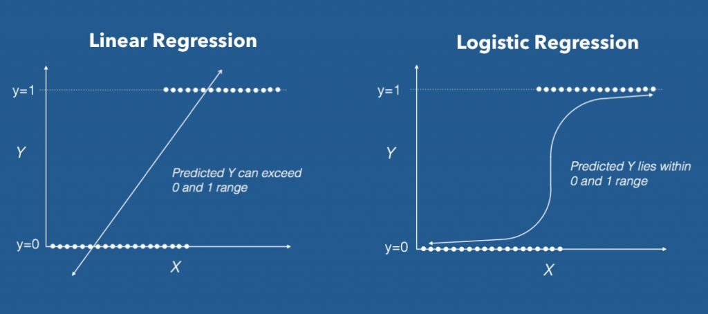
Lojistik regresyon, bağımlı değişkenin iki kategorili (örneğin: evet/hayır, hasta/sağlıklı) olduğu durumlarda kullanılan bir istatistiksel modeldir. Bu yöntem, olasılıkları tahmin ederek verinin belirli bir sınıfa ait olup olmadığını belirlemeye yarar. Lineer regresyondan farklı olarak, sonuçları 0 ile 1 arasında bir olasılık değeri olarak verir.

Özgür Nurettin Öztürk 29 Haziran 2025 6 dk

İstatistik
Makine Öğrenmesi

Lojistik regresyon, özellikle sınıflandırma problemlerinde kullanılan bir istatistiksel modelleme yöntemidir. Bağımlı değişkenin kategorik olduğu durumlarda, özellikle ikili (binary) sonuçlar içeren veri setlerinde yaygın olarak tercih edilir. Örneğin, bir hastanın hasta olup olmadığını, bir e-postanın spam olup olmadığını ya da bir müşterinin ürünü alıp almayacağını tahmin etmek gibi durumlar lojistik regresyonla analiz edilebilir.

Lojistik regresyonun amacı, iki yönlü karakteristiği (bağımlı değişken = yanıt veya sonuç değişkeni) ile ilgili bir dizi bağımsız (öngörücü veya açıklayıcı) değişken arasındaki ilişkiyi tanımlamak için en uygun (henüz biyolojik olarak makul) modeli bulmaktır. Lojistik regresyon, ilgi karakteristiklerinin varlığının olasılığını logit dönüşümünü tahmin etmek için bir formülün katsayılarını (standart hatalarını ve önem seviyelerini) üretir.

UYGULAMA ALANLARI

Lojistik regresyon, birçok alanda yaygın olarak kullanılmaktadır:

Sağlık: Bir hastanın belirli bir hastalığı taşıyıp taşımadığını tahmin etmek.
Pazarlama: Bir müşterinin kampanyaya yanıt verip vermeyeceğini öngörmek.
Finans: Bir kişinin kredi geri ödemesini yapıp yapamayacağını tahmin etmek.
Sosyal Bilimler: Anket sonuçlarına göre bireylerin davranışlarını modellemek.
Spam Filtreleme: Bir e-postanın spam olup olmadığını sınıflandırma.

Lojistik Regresyon, diğer gelişmiş sınıflandırma algoritmalarının (SVM, Karar Ağaçları, Sinir Ağları) temelini anlamak için de harika bir başlangıç noktasıdır.

Avantajları ve Dezavantajları

Avantajları:

Basit ve Hızlı: Uygulaması ve eğitilmesi oldukça kolay ve hızlıdır.
Yorumlanabilirlik: Modelin katsayıları (ağırlıkları) kolayca yorumlanabilir. Bir özelliğin katsayısı, o özelliğin çıktı olasılığı üzerindeki etkisini gösterir.
Olasılık Çıktısı: Sonuç olarak sadece bir sınıf etiketi değil, aynı zamanda bu sınıfa ait olma olasılığını da verir.

Dezavantajları:

Doğrusallık Varsayımı: Özellikler ve çıktı değişkeni arasında doğrusal bir ilişki olduğunu varsayar (Sigmoid'den önceki z kısmı). Karmaşık, doğrusal olmayan ilişkileri modellemede zorlanabilir.
Aşırı Uçlara Duyarlılık: Tıpkı Doğrusal Regresyon gibi, aşırı uç (outlier) değerlere karşı hassastır.
Özellik Ölçeklemesi: Farklı ölçeklere sahip özellikler, modelin performansını olumsuz etkileyebilir. Bu nedenle özelliklerin ölçeklenmesi (normalizasyon) genellikle önerilir.

TEORİK TEMELLERİ

Lojistik regresyon, lineer regresyonun bir türevi gibi düşünülebilir, ancak önemli bir farkı vardır: Lineer regresyon sonuçları sürekli sayılarla ifade ederken, lojistik regresyon sonuçları 0 ile 1 arasında bir olasılık değeri üretir. Bu olasılık değeri, belirli bir koşulun gerçekleşme ihtimalini gösterir. Model, bu olasılığı tahmin etmek için "lojistik (sigmoid) fonksiyon" adı verilen S şeklinde bir fonksiyon kullanır.

Nasıl Çalışır

Lojistik Regresyon'un çalışma mekanizması iki ana adımdan oluşur:

1. Doğrusal Modelin Oluşturulması

Öncelikle, tıpkı Doğrusal Regresyon'da olduğu gibi, girdi özelliklerinin ( x1, x2, ... , xn ) ağırlıklı toplamı hesaplanır:

z = w_0 + w_1x_1 + w_2x_2 + \ldots + w_nx_n

Burada:

z: Doğrusal modelin çıktısı
w0: Kesme noktası (Bias)
wi: Her bir özelliğin ağırlığı (katsayısı)
xi: Giriş özellikleri (features)

2. Sigmoid Fonksiyonu (Lojistik Fonksiyon)

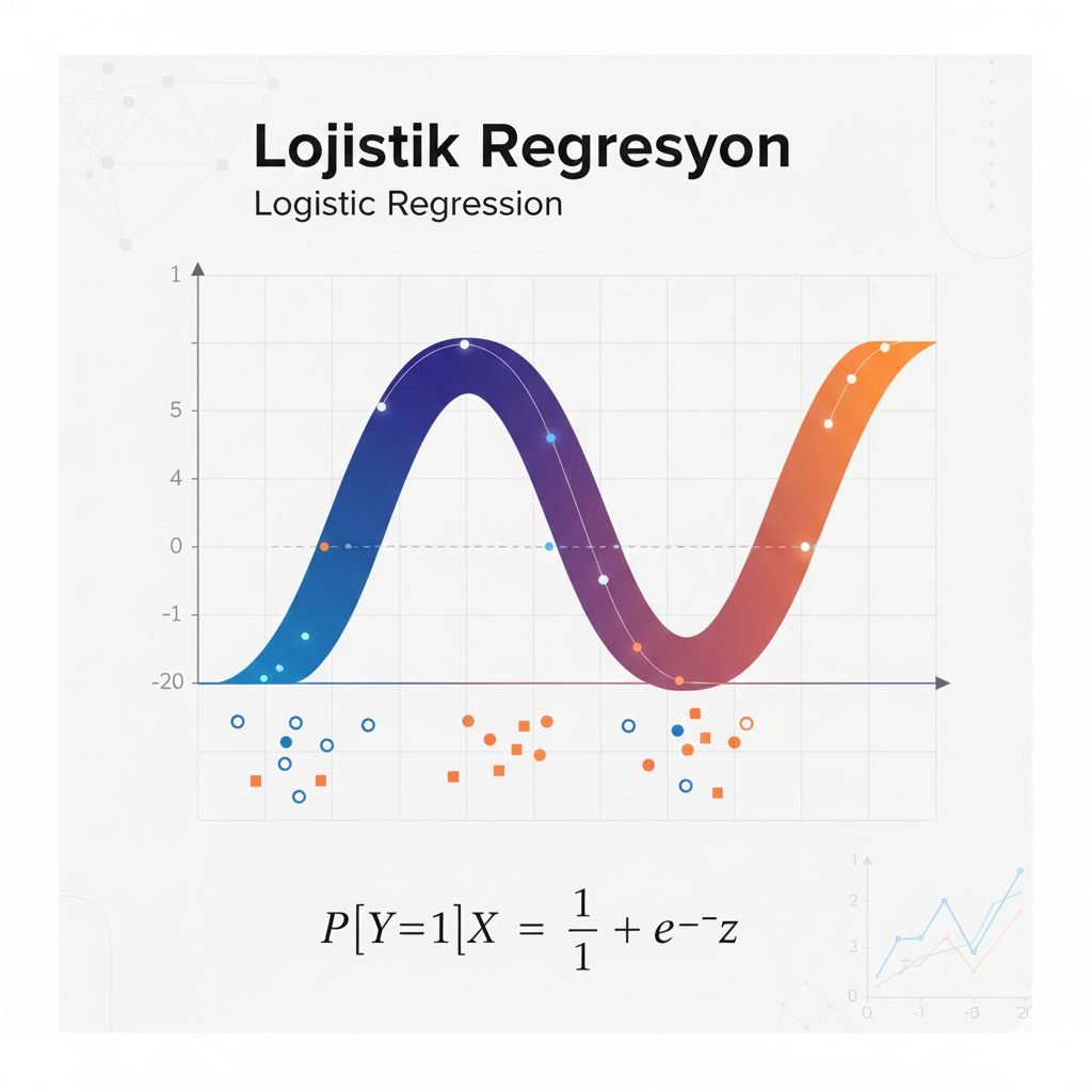
Doğrusal modelin çıktısı olan z, - ∞ile +∞ arasında herhangi bir değer alabilir. Sınıflandırma için bu değeri bir olasılığa çevirmemiz gerekir. İşte bu noktada Sigmoid Fonksiyonu ( h(z) ) devreye girer.

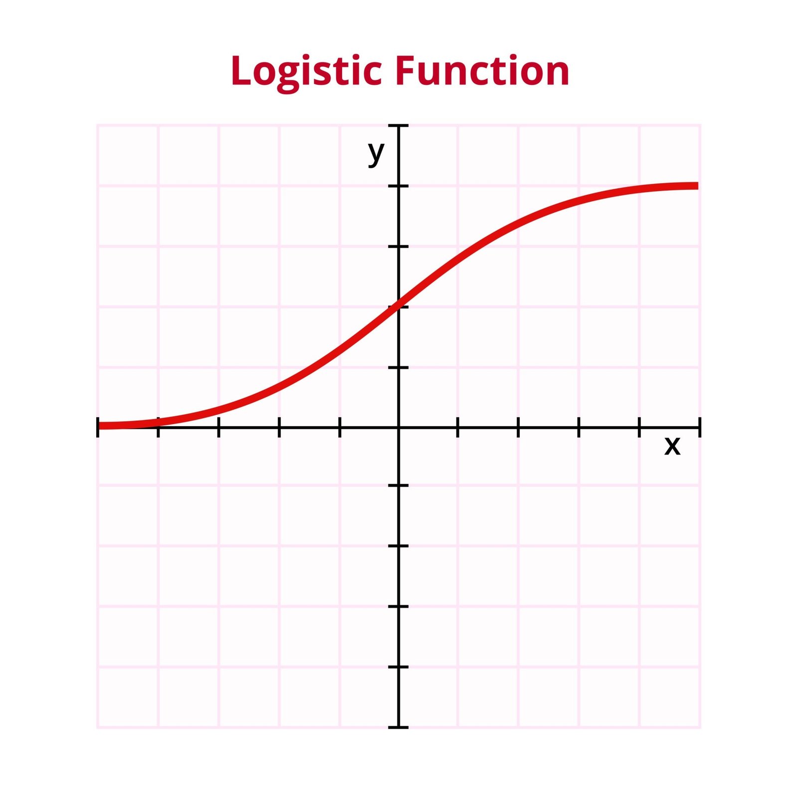
Sigmoid fonksiyonu, z değerini 0 ile 1 arasına sıkıştırır ve bize pozitif sınıfa ait olma olasılığını verir:

P(Y=1 \mid X) = h(z) = \frac{1}{1+e^{-z}}

Bu olasılık değeri, tahmin edilen sınıfı belirlemek için bir eşikle (genellikle 0.5) karşılaştırılır:

Eğer P(Y=1|X) ≥ 0,5 ise, tahmin edilen sınıf 1'dir.
Eğer P(Y=1|X) < 0,5 ise, tahmin edilen sınıf 0'dır.

Model Eğitimi (Maliyet Fonksiyonu)

Lojistik Regresyon'da, modelin ağırlıklarını (wi) optimize etmek için Maksimum Olabilirlik Tahmini (Maximum Likelihood Estimation - MLE) kullanılır. Bu, verilen ağırlıklarla gözlemlenen veri kümesini elde etme olasılığını maksimize etmeye eşdeğerdir.

Bunu yapmak için, genellikle Çapraz Entropi (Cross-Entropy) veya Log Kaybı (Log Loss) olarak bilinen bir maliyet fonksiyonu kullanılır. Bu fonksiyon, tahmin edilen olasılık ile gerçek etiket arasındaki farkı cezalandırır:

J(\mathbf{w}) = -\frac{1}{m}\sum_{i=1}^{m}\left[\, y^{(i)}\log\!\left(h(z^{(i)})\right) + \left(1-y^{(i)}\right)\log\!\left(1-h(z^{(i)})\right) \right]

yi: Gerçek etiket (0 veya 1).
h(z^i): Tahmin edilen olasılık.
m: Eğitim örneklerinin sayısı.

Model, bu maliyet fonksiyonunu Gradyan İnişi (Gradient Descent) gibi optimizasyon algoritmaları kullanarak minimize edecek ağırlık (wi) değerlerini öğrenir.

Katsayıların Yorumlanabilirliği (Odds Oranı)

Lojistik Regresyon'un en güçlü yanlarından biri, her bir özellik için öğrenilen ağırlıkların ( $w_i$ ) bize bu özelliğin olasılık üzerindeki etkisini net bir şekilde söylemesidir.

Doğrusal regresyonda katsayılar doğrudan $Y$ üzerindeki etkiyi gösterirken, Lojistik Regresyon'da katsayılar Odds Oranı (Odds Ratio) üzerinden yorumlanır.

Odds Nedir?

Odds (Oran), bir olayın gerçekleşme olasılığının ( $P$ ), gerçekleşmeme olasılığına ( $1-P$ ) bölünmesiyle bulunur:

\text{Odds} = \frac{P}{1-P}

Odds Oranı ve Katsayılar (wi)

Bir özelliğin katsayısı ( $w_i$ ) ne kadar büyük ve pozitifse, o özellik pozitif sınıfın (1) olasılığını o kadar artırır. Bu ilişkiyi anlamak için $w_i$ 'nin üstelini (e^wi) alırız.

e^wi değeri, ilgili xi özelliğinin bir birim artmasının, Odds Oranını kaç kat artırdığını gösterir.

$e^{w_i}$ Değeri	Yorum	Etki
$e^{w_i} > 1$	Özellik $x_i$ arttığında, Odds Oranı katlanarak artar.	Pozitif Etki (Sınıf 1 olasılığını artırır)
$e^{w_i} = 1$	Özellik $x_i$ ’nin bir etkisi yoktur.	Nötr Etki
$e^{w_i} < 1$	Özellik $x_i$ arttığında, Odds Oranı azalır.	Negatif Etki (Sınıf 1 olasılığını azaltır)

Model Uyum İstatistikleri (Goodness of Fit)

Bu istatistikler, modelin gözlemlenen verilere ne kadar iyi uyduğunu ölçer.

1. Olabilirlik Oranı Testi (Likelihood Ratio Test)

Amaç: Modelin, sadece kesme terimini içeren (null) modele göre anlamlı bir gelişme sağlayıp sağlamadığını test eder.
İstatistik: X^2 (Ki-kare) dağılımına sahip olan Olabilirlik Oranı X^2 İstatistiği kullanılır.

\chi^2 = -2 \cdot \log(\text{Olabilirlik Oranı}) = -2 \cdot \left(\text{Log Olabilirlik}_{\text{Null}} - \text{Log Olabilirlik}_{\text{Model}}\right)

P-Değeri: Eğer X^2 istatistiğinin p-değeri (genellikle 0.05'ten) küçükse, modelin genel olarak anlamlı olduğu ve yordayıcıların modele katkıda bulunduğu sonucuna varılır.

2. Pseudo R^2 Metrikleri

Doğrusal regresyondaki R^2 (Açıklanan Varyans Oranı) metriğinin bir karşılığıdır, ancak Lojistik Regresyon'da tam olarak aynı şekilde yorumlanmaz. Modelin, null modele kıyasla açıklamadaki iyileşmesini gösterir.

Cox ve Snell R^2:
Nagelkerke R^2: En sık kullanılan Pseudo R^2 metriğidir ve maksimum değeri 1 olacak şekilde normalize edilmiştir. Yüksek bir değer (0.20 ve üzeri kabul edilebilir sayılabilir) daha iyi bir uyum anlamına gelir.

3. Hosmer-Lemeshow Testi

Amaç: Modelin kalibrasyonunu, yani tahmin edilen olasılıkların gerçekleşen sonuçlara ne kadar uyduğunu kontrol etmek için kullanılan bir uyum testidir.
İstatistik: Gözlenen ve beklenen olay sayıları arasındaki farkları özetleyen bir X^2 istatistiği hesaplanır.
Yorum: Büyük bir p-değeri (genellikle 0.05'ten büyük) iyi bir uyum gösterir, çünkü null hipotez (modelin iyi bir uyuma sahip olduğu) reddedilemez.

Logistic regression is a statistical modeling method used especially for classification problems. It is widely preferred when the dependent variable is categorical, particularly for data sets with binary outcomes. For example, predicting whether a patient is sick, whether an email is spam, or whether a customer will buy a product can all be analyzed with logistic regression.

The goal of logistic regression is to find the best-fitting (yet biologically reasonable) model to describe the relationship between a dichotomous characteristic of interest (the dependent variable = response or outcome variable) and a set of independent (predictor or explanatory) variables. Logistic regression generates the coefficients (with their standard errors and significance levels) of a formula that predicts a logit transformation of the probability that the characteristic of interest is present.

APPLICATION AREAS

Logistic regression is widely used in many fields:

Healthcare: Predicting whether a patient has a particular disease.
Marketing: Predicting whether a customer will respond to a campaign.
Finance: Predicting whether a person will repay a loan.
Social Sciences: Modeling individuals' behavior based on survey results.
Spam Filtering: Classifying whether an email is spam or not.

Logistic regression is also a great starting point for understanding the foundations of other advanced classification algorithms (SVM, decision trees, neural networks).

Advantages and Disadvantages

Advantages:

Simple and Fast: It is quite easy and fast to implement and train.
Interpretability: The model's coefficients (weights) are easy to interpret. A feature's coefficient shows its effect on the output probability.
Probability Output: It returns not only a class label but also the probability of belonging to that class.

Disadvantages:

Linearity Assumption: It assumes a linear relationship between the features and the output (the z part before the sigmoid). It can struggle to model complex, non-linear relationships.
Sensitivity to Outliers: Just like linear regression, it is sensitive to outliers.
Feature Scaling: Features on different scales can hurt the model's performance, so feature scaling (normalization) is generally recommended.

THEORETICAL FOUNDATIONS

Logistic regression can be thought of as a variant of linear regression, but with one important difference: linear regression expresses results as continuous numbers, whereas logistic regression produces a probability between 0 and 1. This probability shows how likely a given condition is to occur. To estimate it, the model uses an S-shaped function called the "logistic (sigmoid) function".

How It Works

The logistic regression mechanism consists of two main steps:

1. Building the Linear Model

First, just as in linear regression, the weighted sum of the input features ( x1, x2, ... , xn ) is computed:

z = w_0 + w_1x_1 + w_2x_2 + \ldots + w_nx_n

Where:

z: Output of the linear model
w0: Intercept (bias)
wi: Weight (coefficient) of each feature
xi: Input features

2. Sigmoid Function (Logistic Function)

The output of the linear model, z, can take any value between −∞ and +∞. For classification, we need to turn this value into a probability. This is where the Sigmoid Function ( h(z) ) comes in.

The sigmoid function squeezes z into the range 0 to 1 and gives us the probability of belonging to the positive class:

P(Y=1 \mid X) = h(z) = \frac{1}{1+e^{-z}}

This probability is compared with a threshold (usually 0.5) to determine the predicted class:

If P(Y=1|X) ≥ 0.5, the predicted class is 1.
If P(Y=1|X) < 0.5, the predicted class is 0.

Model Training (Cost Function)

In logistic regression, the model's weights (wi) are optimized using Maximum Likelihood Estimation (MLE) . This is equivalent to maximizing the probability of obtaining the observed data set with the given weights.

To do this, a cost function commonly known as Cross-Entropy or Log Loss is used. This function penalizes the difference between the predicted probability and the true label:

J(\mathbf{w}) = -\frac{1}{m}\sum_{i=1}^{m}\left[\, y^{(i)}\log\!\left(h(z^{(i)})\right) + \left(1-y^{(i)}\right)\log\!\left(1-h(z^{(i)})\right) \right]

yi: True label (0 or 1).
h(z^i): Predicted probability.
m: Number of training examples.

The model learns the weight (wi) values that minimize this cost function using optimization algorithms such as Gradient Descent .

Interpretability of the Coefficients (Odds Ratio)

One of the strongest aspects of logistic regression is that the learned weights ( $w_i$ ) tell us clearly how each feature affects the probability.

In linear regression the coefficients directly show the effect on $Y$ , whereas in logistic regression the coefficients are interpreted through the Odds Ratio .

What Are Odds?

Odds are found by dividing the probability that an event occurs ( $P$ ) by the probability that it does not occur ( $1-P$ ):

\text{Odds} = \frac{P}{1-P}

Odds Ratio and Coefficients (wi)

The larger and more positive a feature's coefficient ( $w_i$ ) is, the more that feature increases the probability of the positive class (1). To understand this relationship, we take the exponential of $w_i$ (e^wi).

The e^wi value shows how many times the odds ratio is multiplied when the related feature xi increases by one unit.

$e^{w_i}$ Value	Interpretation	Effect
$e^{w_i} > 1$	As feature $x_i$ increases, the odds ratio grows multiplicatively.	Positive effect (increases the probability of class 1)
$e^{w_i} = 1$	Feature $x_i$ has no effect.	Neutral effect
$e^{w_i} < 1$	As feature $x_i$ increases, the odds ratio decreases.	Negative effect (decreases the probability of class 1)

Model Fit Statistics (Goodness of Fit)

These statistics measure how well the model fits the observed data.

1. Likelihood Ratio Test

Purpose: Tests whether the model provides a significant improvement over the null model that contains only the intercept.
Statistic: The likelihood ratio X^2 statistic, which follows an X^2 (chi-square) distribution, is used.

\chi^2 = -2 \cdot \log(\text{Likelihood Ratio}) = -2 \cdot \left(\text{Log-Likelihood}_{\text{Null}} - \text{Log-Likelihood}_{\text{Model}}\right)

P-Value: If the p-value of the X^2 statistic is smaller than the threshold (usually 0.05), the model is considered significant overall and the predictors contribute to the model.

2. Pseudo R^2 Metrics

They are counterparts of the R^2 (proportion of explained variance) metric in linear regression, but they are not interpreted in exactly the same way in logistic regression. They show how much the model improves on the null model.

Cox and Snell R^2:
Nagelkerke R^2: The most commonly used Pseudo R^2 metric, normalized so that its maximum value is 1. A higher value (0.20 and above can be considered acceptable) indicates a better fit .

3. Hosmer-Lemeshow Test

Purpose: A goodness-of-fit test used to check the model's calibration, i.e. how well the predicted probabilities match the observed outcomes.
Statistic: An X^2 statistic summarizing the differences between observed and expected event counts is calculated.
Interpretation: A large p-value (usually greater than 0.05) indicates a good fit , because the null hypothesis (that the model fits well) cannot be rejected.

Avantajları ve Dezavantajları

Avantajları:

Nasıl Çalışır

Model Uyum İstatistikleri (Goodness of Fit)

Advantages and Disadvantages

Advantages:

How It Works

Model Fit Statistics (Goodness of Fit)

Diğer Yazılar

Karar Ağacı / CART

Normal Dağılım

Belirtme Katsayısı