Python ile Aykırı Değer Tespiti
Uç değerler her zaman hata değildir; çoğu zaman en çok şey anlatan kayıtlardır. IQR, Z-skoru, MAD ve Isolation Forest'ı karşılaştırıyor, hangisinin nerede işe yaradığını ve aday listesiyle ne yapılması gerektiğini anlatıyorum.
- Araçlar
- İstatistik
Aykırı değer nedir?
Genel örüntüden uzak duran bir gözlem, mutlaka veri hatası değildir. Ölçüm yanlışı olabilir; nadir ama gerçekten yaşanmış bir olay olabilir; ya da verinin içinde ayrı bir alt grup bulunduğunun işareti olabilir. Üçü de farklı kararlar gerektirir.
Uç değerler ortalamayı, standart sapmayı, regresyon katsayılarını ve uzaklık temelli modelleri belirgin biçimde etkiler. Tek bir hatalı kayıt, binlerce satırlık bir veri setinin ortalamasını gözle görülür biçimde kaydırabilir.
1. Önce veriyi keşfedin
Değişkenin türünü, birimini ve dağılımını anlamadan eşik belirlemeyin. Histogram, kutu grafiği ve — zaman boyutu varsa — zaman grafiğini özet istatistiklerle birlikte okuyun. Fiziksel ve iş sınırlarını da doğrulayın: negatif bir süre ya da %150 oran, hiçbir istatistiksel teste gerek kalmadan hatadır.
import pandas as pd
import seaborn as sns
import matplotlib.pyplot as plt

df = pd.read_csv("olcumler.csv")
x = df["deger"].dropna()

print(x.describe(percentiles=[.01, .25, .5, .75, .99]))

sns.histplot(x, kde=True)
plt.show()
percentiles listesine %1 ve %99'u eklemek işe yarar: uçların nerede başladığını, en büyük değere bakmadan önce görmenizi sağlar.
2. IQR: çeyrekler arası aralık
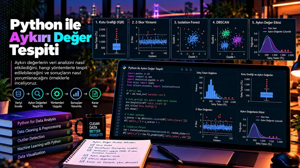
IQR = Q3 − Q1. Tukey kuralı, Q1 − 1,5 × IQR altındaki ve Q3 + 1,5 × IQR üstündeki değerleri aday sayar. Yöntemin en büyük avantajı normal dağılım varsaymamasıdır; çarpık dağılımlarda da çalışır.
q1, q3 = x.quantile([.25, .75])
iqr = q3 - q1
alt, ust = q1 - 1.5 * iqr, q3 + 1.5 * iqr

aday = df.loc[df["deger"].lt(alt) | df["deger"].gt(ust)]
print(len(aday), "aday kayıt")
1,5 katsayısı bir gelenektir, doğa yasası değil. Daha temkinli bir tarama için 3,0 kullanılır. Eşiği veriye ve analizin amacına göre seçin; seçtiğiniz değeri de raporlayın.
3. Z-skoru
Z-skoru, bir gözlemin ortalamadan uzaklığını standart sapma biriminde ölçer. |z| > 3 yaygın bir uyarı eşiğidir ve yaklaşık normal, simetrik dağılımlarda anlamlıdır.
std = x.std(ddof=0)
z = (x - x.mean()) / std if std else x * 0

aday_z = df.loc[z.abs().gt(3)]4. MAD ile sağlam Z-skoru
Medyan mutlak sapma (MAD), medyandan uzaklıkların medyanıdır. Hem merkez hem yayılım ölçüsü olarak medyan kullandığı için uçlardan çok daha az etkilenir.
med = x.median()
mad = (x - med).abs().median()

if mad:
    rz = .6745 * (x - med) / mad
    aday_mad = df.loc[rz.abs().gt(3.5)]
Koddaki 0.6745 sabiti MAD'i normal dağılımda standart sapmayla karşılaştırılabilir ölçeğe getirir; bu sayede 3,5 eşiği z-skorundaki 3 eşiğiyle benzer anlam taşır. if mad: kontrolü de gereksiz değil: veri setinde aynı değer çok tekrar ediyorsa MAD sıfır çıkar ve bölme işlemi patlar.
5. Çok değişkenli tespit
Her sütuna tek tek bakıldığında tamamen olağan görünen bir kayıt, değişkenler arasındaki ilişkiye göre sıra dışı olabilir. 2 adet ürün için 50.000 TL tutar, ne adet ne de tutar sütununda uç değildir — ama ikisi birlikte dikkat çeker.
from sklearn.ensemble import IsolationForest

X = df[["tutar", "adet", "sure"]].dropna()

model = IsolationForest(contamination=.02, random_state=42)
etiket = model.fit_predict(X)        # -1 = aday
skor = model.decision_function(X)   # düşük skor = daha anormal
contamination modele "veride kabaca ne oranda aykırı değer bekliyorsun" diye sorar; cevabınız doğrudan kaç kayıt işaretleneceğini belirler. Bu yüzden onu bir keşif parametresi gibi kullanın: birkaç farklı değerde çalıştırıp hangi kayıtların her ayarda işaretlendiğine bakın. Her seferinde çıkanlar, gerçekten ilgilenmeniz gereken kayıtlardır.
Hangi yöntem, ne zaman?
| Yöntem | Uygun kullanım | Sınırlama |
|---|---|---|
| IQR | Tek değişken, çarpık dağılım | Alt grupları kaçırabilir |
| Z-skoru | Yaklaşık normal dağılım | Uçların kendisinden etkilenir |
| MAD | Sağlam tek değişkenli tarama | Tekrar eden değerlerde sıfır olur |
| Isolation Forest | Çok değişkenli örüntü | Parametre ayarı gerektirir |
Pratikte en iyi yaklaşım tek bir yönteme bağlanmak değil, iki veya üçünü birlikte çalıştırıp kesişime bakmaktır. Hem IQR'ın hem MAD'in hem de Isolation Forest'ın işaretlediği bir kayıt, yalnızca birinin işaretlediğinden çok daha güçlü bir adaydır.
6. Sonuçları yorumlayın
- Hata
Araştır - Bağlamı
Değerlendir - Alt Grupları
Karşılaştır - Etkiyi
Ölç - Kararı
Belgele
- Ölçüm, aktarım ve birim hatalarını araştırın. TL ile kuruş, metre ile santimetre karışıklığı en sık rastlanan nedendir.
- Kampanya, iade, arıza ve mevsimselliği değerlendirin. Uç değer çoğu zaman gerçek bir olayın izidir.
- Alt grupları ve dönemleri karşılaştırın. Bir segmentte normal olan, tüm veride uç görünebilir.
- Adaylar dahil ve hariç analizi ayrı ayrı çalıştırın. Sonuç değişmiyorsa tartışma kapanır; değişiyorsa kararınızı raporda açıklamanız gerekir.
- Kararı ve gerekçesini belgeleyin. Hangi kayıt neden çıkarıldı sorusunun cevabı kodda değil, raporda olmalı.
Kontrol listesi
Sınırları doğrula
Birim ve iş kurallarına göre imkânsız değerleri istatistik öncesinde ayıklayın.
Grafikle bak
Histogram ve kutu grafiği, hiçbir eşiğin göstermeyeceği şekil bilgisini verir.
Yöntemi veriye göre seç
Çarpık dağılımda z-skoru, tekrar eden değerlerde MAD sorun çıkarır.
Otomatik silme
Hiçbir eşik tek başına silme yetkisi vermez; aday listesi incelenmek içindir.
Etkiyi denetle
Adaylar dahil ve hariç sonuçları karşılaştırın; fark varsa bu da bir bulgudur.
Eşiği raporla
Hangi yöntem, hangi eşik ve kaç kayıt — üçü de raporda yazılı olsun.
Tespit bir süreçtir, hüküm değil
Aykırı değer tespiti tek bir formülün kesin hükmü değil, incelenecek gözlemleri bulma sürecidir. IQR, z-skoru, MAD ve Isolation Forest size aday listesi verir; bu listenin ne anlama geldiğini veri kaynağı ve analizin amacı belirler.
En maliyetli hata, uçları otomatik silen bir temizleme adımı yazıp bir daha dönüp bakmamaktır. Çünkü silinen kayıtlar çoğu zaman en çok şey anlatan kayıtlardır: büyük bir müşteri, bir sistem arızası, bir kampanya günü ya da düzeltilmesi gereken gerçek bir veri hatası.
What is an outlier?
An observation far from the general pattern is not necessarily a data error. It may be a measurement mistake; it may be a rare but genuine event; or it may be a sign that the data contains a separate subgroup. All three call for different decisions.
Extreme values markedly affect the mean, the standard deviation, regression coefficients and any distance-based model. A single bad record can visibly shift the average of a dataset with thousands of rows.
1. Explore the data first
Do not set a threshold before understanding the variable's type, unit and distribution. Read the histogram, the box plot and — if there is a time dimension — the time plot together with the summary statistics. Verify the physical and business limits too: a negative duration or a 150% rate is an error without any statistical test.
import pandas as pd
import seaborn as sns
import matplotlib.pyplot as plt

df = pd.read_csv("olcumler.csv")
x = df["deger"].dropna()

print(x.describe(percentiles=[.01, .25, .5, .75, .99]))

sns.histplot(x, kde=True)
plt.show()
Adding the 1st and 99th percentiles to the percentiles list is worth it: it shows you where the tails begin before you look at the maximum.
2. IQR: the interquartile range
IQR = Q3 − Q1. Tukey's rule flags values below Q1 − 1.5 × IQR and above Q3 + 1.5 × IQR as candidates. Its biggest advantage is that it assumes no normal distribution, so it works on skewed data too.
q1, q3 = x.quantile([.25, .75])
iqr = q3 - q1
alt, ust = q1 - 1.5 * iqr, q3 + 1.5 * iqr

aday = df.loc[df["deger"].lt(alt) | df["deger"].gt(ust)]
print(len(aday), "candidate records")
The 1.5 multiplier is a convention, not a law of nature. A more conservative scan uses 3.0. Choose the threshold according to the data and the purpose of the analysis — and report the value you chose.
3. The Z-score
A Z-score measures an observation's distance from the mean in units of standard deviation. |z| > 3 is a common warning threshold and is meaningful on roughly normal, symmetric distributions.
std = x.std(ddof=0)
z = (x - x.mean()) / std if std else x * 0

aday_z = df.loc[z.abs().gt(3)]4. A robust Z-score with MAD
The median absolute deviation (MAD) is the median of the distances from the median. Because it uses the median for both centre and spread, it is far less affected by the tails.
med = x.median()
mad = (x - med).abs().median()

if mad:
    rz = .6745 * (x - med) / mad
    aday_mad = df.loc[rz.abs().gt(3.5)]
The 0.6745 constant rescales MAD so that it is comparable to the standard deviation under a normal distribution; that is what makes the 3.5 threshold carry a similar meaning to the 3 used with Z-scores. The if mad: check is not redundant either: if one value repeats often enough, MAD comes out as zero and the division fails.
5. Multivariate detection
A record that looks entirely ordinary in every single column can be unusual given the relationship between the columns. A total of 50,000 for 2 items is extreme in neither the quantity nor the amount column — but the combination stands out.
from sklearn.ensemble import IsolationForest

X = df[["tutar", "adet", "sure"]].dropna()

model = IsolationForest(contamination=.02, random_state=42)
etiket = model.fit_predict(X)        # -1 = candidate
skor = model.decision_function(X)   # lower score = more anomalous
contamination asks the model roughly what proportion of outliers you expect, and your answer directly determines how many records get flagged. So treat it as an exploratory parameter: run it at several values and see which records are flagged at every setting. Those are the ones genuinely worth your attention.
Which method, and when?
| Method | Suitable for | Limitation |
|---|---|---|
| IQR | One variable, skewed distribution | Can miss subgroups |
| Z-score | Roughly normal distribution | Affected by the tails themselves |
| MAD | Robust single-variable scanning | Becomes zero with repeated values |
| Isolation Forest | Multivariate patterns | Needs parameter tuning |
In practice the best approach is not committing to one method but running two or three and looking at the intersection. A record flagged by IQR, MAD and Isolation Forest alike is a far stronger candidate than one flagged by a single method.
6. Interpret the results
- Investigate
Errors - Weigh the
Context - Compare
Subgroups - Measure the
Impact - Document the
Decision
- Investigate measurement, transfer and unit errors. Mixing currency with sub-units, or metres with centimetres, is the most common cause.
- Weigh campaigns, returns, outages and seasonality. An extreme value is often the trace of a real event.
- Compare subgroups and periods. What is normal within one segment can look extreme across the whole dataset.
- Run the analysis both with and without the candidates. If the result does not change, the debate is over; if it does, your decision has to be explained in the report.
- Document the decision and its reasoning. Which record was removed and why belongs in the report, not only in the code.
A checklist
Verify the limits
Filter out values impossible under the unit and the business rules before any statistics.
Look at the plot
Histograms and box plots carry shape information no threshold will ever show you.
Match method to data
Z-scores struggle on skewed data; MAD breaks down when values repeat.
No automatic deletion
No threshold grants permission to delete; a candidate list exists to be reviewed.
Audit the impact
Compare results with and without the candidates; a difference is itself a finding.
Report the threshold
Which method, which threshold and how many records — all three belong in the report.
Detection is a process, not a verdict
Outlier detection is not the final word of a single formula; it is the process of finding the observations worth examining. IQR, Z-scores, MAD and Isolation Forest hand you a candidate list — what that list means is decided by the data source and the purpose of the analysis.
The most expensive mistake is writing a cleaning step that silently deletes the extremes and never looking again. Because the deleted records are often the ones with the most to say: a major customer, a system failure, a campaign day, or a genuine data error that needed fixing.