Zaman Serisi Analizine Giriş: Bileşenler, Durağanlık ve ARIMA
Serinin bileşenlerine ayrılmasından durağanlığa, ACF ve PACF'ten ARIMA ile tahmine kadar zaman serisi analizinin temellerini R örnekleriyle inceliyorum.
- İstatistik
- Araçlar

Bir sayı dizisine zaman damgası eklendiği anda problem değişir. Artık gözlemler birbirinden bağımsız değildir: bugünkü değer dünkünden, bu ayki değer geçen yılın aynı ayından etkilenir. Klasik regresyonun dayandığı “gözlemler bağımsızdır” varsayımı burada çöker ve veriye özel bir araç setine ihtiyaç duyulur.
Bu yazıda zaman serisi analizinin temel kavramlarını R üzerinden ele alıyorum: serinin bileşenlerine ayrılması, durağanlık, otokorelasyon ve ARIMA ile tahmin. Örnekler R ile birlikte gelen nottem veri setinden geliyor; ek dosya indirmeden kendi makinende tekrarlayabilirsin.
“Zaman serisi analizinde asıl soru ‘hangi model daha iyi?’ değil, ‘bu serinin hangi bölümü sistematik, hangi bölümü rastlantı?’ sorusudur.”
1. Zaman Serisi Nedir?
Zaman serisi, bir değişkene ait gözlemlerin zaman sırasına göre dizilmesiyle oluşan veridir. T örneklem büyüklüğü olmak üzere genellikle Xt, t = 1, 2, …, T biçiminde gösterilir.
Sürekli
Zaman içinde kesintisiz kaydedilebilen veriler: elektrik sinyali, titreşim.
Kesikli
Yalnızca belirli anlarda elde edilen veriler: faiz oranı, aylık satış hacmi.
Düzenli
Gözlemler arasındaki süre eşittir: her gün, her ay, her çeyrek.
Düzensiz
Gözlem aralıkları eşit değildir; çoğu yöntem önce düzenli hale getirmeyi gerektirir.
R'da bir vektörü zaman serisine çeviren şey ts sınıfı ve onun frekans bilgisidir. Frekans, bir mevsimsel döngüde kaç gözlem olduğunu söyler: aylık veride 12, çeyreklik veride 4. Bu tek sayı, ilerideki bütün mevsimsellik hesaplarının dayanağıdır.
library(tidyverse)
library(forecast)
library(tseries)

# nottem: Nottingham Kalesi aylik ortalama hava sicakligi (°F), 1920-1939
class(nottem)      # "ts"
frequency(nottem)  # 12 -> aylik
start(nottem)      # 1920 1

autoplot(nottem) +
  labs(title = "Nottingham aylık ortalama sıcaklık",
       x = "Yıl", y = "Sıcaklık (°F)")
2. Serinin Bileşenleri
Bir zaman serisi, matematiksel olarak formüle edilebilen deterministik öğelerle rassal süreçlerden doğan stokastik öğelerin toplamıdır. Klasik ayrıştırma bu yapıyı dört bileşene indirger.
| Bileşen | Gösterim | Ne anlatır? |
|---|---|---|
| Trend | T | Serinin uzun dönemli yükselme veya alçalma eğilimi. |
| Mevsimsellik | S | Sabit periyotla tekrar eden dalgalanma (yılın ayları, haftanın günleri). |
| Konjonktür | C | Mevsimsellikten uzun, sabit periyodu olmayan dalgalar; ekonomik çevrimler. |
| Düzensiz / rassal | I | Geri kalan her şey: açıklanamayan kısım. |
Bu bileşenler iki biçimde birleşebilir. Toplamsal model, mevsimsel dalganın genliği serinin seviyesinden bağımsız olduğunda uygundur:
Çarpımsal model ise mevsimsel dalga serinin seviyesiyle birlikte büyüdüğünde kullanılır:
3. Ayrıştırma: decompose()
R'da decompose() hareketli ortalamalarla trendi tahmin eder, trendden arındırılmış seriden mevsimsel ortalamaları çıkarır ve geriye kalanı rassal bileşen olarak verir.
ayrisim <- decompose(nottem)        # varsayilan: type = "additive"
plot(ayrisim)

# Bilesenlere tek tek erisim
ayrisim$trend
ayrisim$seasonal
ayrisim$random

# Carpimsal ayristirma
plot(decompose(nottem, type = "multiplicative"))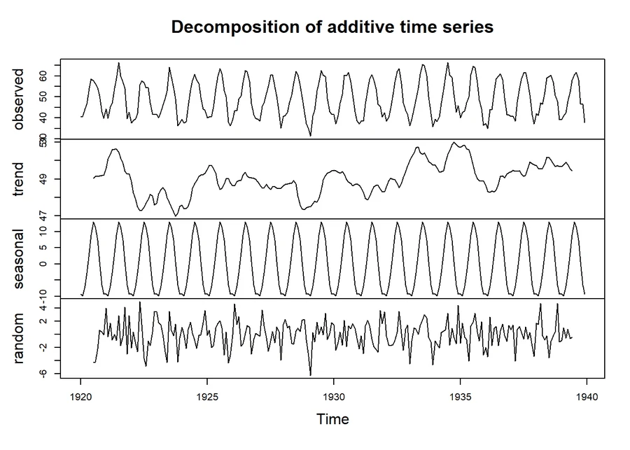
Grafikte dört panel var: gözlenen seri, trend, mevsimsel bileşen ve rassal bileşen. nottem için mevsimsel panel neredeyse birebir tekrar eden bir dalga gösteriyor; trend panelinde ise belirgin bir yön yok, 20 yıl boyunca ortalama sıcaklık dar bir bantta geziniyor.
Mevsimsel dalganın genliği yıllar içinde büyümediği için bu seride toplamsal model doğru tercihtir. Çarpımsal ayrıştırmanın klasik örneği AirPassengers'tır: yolcu sayısı arttıkça yaz–kış farkı da mutlak olarak büyür, dolayısıyla genlik seviyeye bağlıdır.
4. Durağanlık
Durağan (stationary) bir seride ortalama, varyans ve belirli gecikmelerdeki ortak varyans zamana göre değişmez. Yani seriyi hangi dönemden kesip bakarsanız bakın istatistiksel davranışı aynıdır.
Bu neden önemli? Çünkü tahmin yapmanın temeli, geçmişte gözlenen davranışın gelecekte de geçerli olacağı varsayımıdır. Durağan olmayan bir seride bu varsayım çalışmaz; model geçmişe uyar ama geleceği taşımaz. Ayrıca durağan olmayan iki seri arasında, aralarında hiçbir ilişki olmasa bile yüksek R² üreten sahte regresyon ortaya çıkabilir.
Sabit yapı
Ortalama ve varyans zamanla değişmez; şoklar sönümlenir.
Hafızalı
Her değer bir öncekine şok eklenerek oluşur; şokların etkisi kalıcıdır.
Yapısız
Sıfır ortalamalı, sabit varyanslı, gecikmeler arası ilişkisi olmayan seri.
Rassal yürüyüş, durağan olmayan serilerin en bilinen örneğidir:
Burada et ak gürültüdür. Modelin kendisi durağan değildir, çünkü her şok serinin seviyesine kalıcı olarak eklenir. Bir seriyi durağan hale getirmenin en yaygın yolu fark almadır: ardışık gözlemlerin farkına bakmak, rassal yürüyüşü ak gürültüye indirger.
5. Otokorelasyon: ACF ve PACF
Korelasyon iki değişken arasındaki doğrusal ilişkiyi ölçerken, otokorelasyon bir serinin kendi gecikmeli değerleriyle ilişkisini ölçer. rk, seri ile k gecikmeli hali arasındaki ilişkidir:
Bu katsayıların gecikmeye göre çizdirilmiş haline korelogram (ACF) denir. Kısmi otokorelasyon (PACF) ise aradaki gecikmelerin etkisi arındırıldıktan sonra kalan doğrudan ilişkiyi gösterir.
ggAcf(nottem, lag.max = 25) +
  labs(title = "nottem — otokorelasyon (ACF)")

ggPacf(nottem, lag.max = 42) +
  labs(title = "nottem — kısmi otokorelasyon (PACF)")
Grafiklerdeki mavi kesikli çizgiler güven sınırlarıdır. Yorumlarken şunlara bakılır:
| Görünüm | Ne anlama gelir? |
|---|---|
| Çubuklar güven sınırları içinde | İlgili gecikmede anlamlı otokorelasyon yok. |
| Yüksek değerden başlayıp çok yavaş sönen ACF | Seri durağan değil; fark alma gerekebilir. |
| 12, 24, 36… gecikmelerde tekrar eden tepeler | Aylık veride mevsimsellik. |
| ACF q gecikmeden sonra kesiliyor | MA(q) süreci için ipucu. |
| PACF p gecikmeden sonra kesiliyor | AR(p) süreci için ipucu. |
6. Birim Kök ve ADF Testi
Grafik ve korelogram durağanlık hakkında fikir verir ama karar için yetmez. Hassas ölçüm birim kök testleri ile yapılır. Serinin kendi gecikmesiyle açıklandığı modelde katsayının 1 olup olmadığı test edilir:
ρ = 1 ise seri birim köke sahiptir, yani rassal yürüyüş davranışı gösterir ve durağan değildir. Genişletilmiş Dickey-Fuller (ADF) testinin hipotezleri şöyledir:
| Hipotez | İfade |
|---|---|
| H₀ | Seride birim kök vardır (durağan değildir). |
| H₁ | Seride birim kök yoktur (durağandır). |
nottem_random <- decompose(nottem)$random
nottem_random <- na.remove(nottem_random)  # uclardaki NA'lar

tsdisplay(nottem_random)
adf.test(nottem_random) Augmented Dickey-Fuller Test
data: nottem_random
Dickey-Fuller = -8.4454, Lag order = 6, p-value = 0.01
alternative hypothesis: stationaryp-değeri 0,05'in altında olduğu için H₀ reddedilir: mevsimsel ve trend bileşenlerinden arındırılmış seride birim kök yoktur, seri durağandır. Modelleme aşamasına geçilebilir.
tseries paketindeki adf.test() p-değerini bir tabloya göre hesaplar ve tablonun sınırlarında keser. Buradaki 0,01 “tam olarak %1” değil, “%1'den küçük” anlamına gelir; R bu durumda bir uyarı da basar. Ayrıca decompose() sonrası tespit edilen durağanlık ham nottem serisinin durağan olduğu anlamına gelmez — test edilen, arındırılmış seridir.7. AR, MA ve ARMA
Durağan bir seriyi modellemenin iki temel yolu vardır: seriyi kendi geçmişiyle açıklamak veya geçmiş hatalarıyla açıklamak.
AR(p) — Otoregresif süreç. Bugünkü değer, kendi gecikmeli değerlerinin doğrusal birleşimidir:
MA(q) — Hareketli ortalama süreci. Bugünkü değer, geçmiş hata terimlerinin ağırlıklı toplamıdır:
ARMA(p,q). Gerçek serilerin çoğu her iki davranışı birlikte gösterir; Box-Jenkins yaklaşımı bu iki yapıyı birleştirir:
AR mertebesi
Kaç gecikmeli gözlem modele girecek? İpucu PACF'tedir.
MA mertebesi
Kaç gecikmeli hata terimi modele girecek? İpucu ACF'tedir.
Fark derecesi
Seriyi durağan yapmak için kaç kez fark alınacak?
8. ARIMA(p,d,q)
ARMA yalnızca durağan serilerde çalışır. Durağan olmayan serilerde önce fark alınır; bu entegrasyon adımı I(d) modele eklendiğinde ARIMA(p,d,q) elde edilir. Mevsimsel seriler için buna bir de mevsimsel terim grubu eklenir ve model ARIMA(p,d,q)(P,D,Q)[m] biçiminde yazılır; m frekanstır.
Mertebeler elle de denenebilir. Aşağıda nottem için üç farklı model kuruldu:
arima(nottem, order = c(2, 0, 0))
arima(nottem, order = c(0, 0, 3))
arima(nottem, order = c(2, 2, 2))| Model | σ² | Log-olabilirlik | AIC |
|---|---|---|---|
| ARIMA(2,0,0) | 15,87 | −673,30 | 1354,60 |
| ARIMA(0,0,3) | 17,55 | −685,27 | 1380,54 |
| ARIMA(2,2,2) | 25,23 | −721,98 | 1453,96 |
Üçü arasında en düşük AIC'ye sahip model ARIMA(2,0,0). Buradaki mantık şu: AIC hem modelin veriye uyumunu hem de parametre sayısını hesaba katar, dolayısıyla “daha karmaşık model her zaman daha iyidir” tuzağına düşmeyi engeller.
ARIMA(2,2,2)'nin en kötü sonucu vermesi de öğretici. nottem durağan olmayan bir trend taşımıyor; iki kez fark almak seriyi düzeltmek yerine gereksiz gürültü ekliyor. Gereğinden fazla fark almak (overdifferencing) yaygın bir hatadır.
9. auto.arima() ile Model Seçimi
Seri sayısı arttığında veya veri gözle incelenemeyecek kadar büyüdüğünde mertebeleri tek tek denemek pratik değildir. forecast paketindeki auto.arima(), birim kök testleriyle d ve D derecelerini belirler, ardından bilgi kriterine göre p, q, P ve Q için arama yapar.
auto.arima(nottem)

# Denenen modelleri gormek icin
auto.arima(nottem, trace = TRUE)

# Adimli aramayi kapatip genis arama yapmak icin
auto.arima(nottem, trace = TRUE, stepwise = FALSE)Series: nottem
ARIMA(1,0,2)(1,1,2)[12] with drift
sigma^2 estimated as 5.22: log likelihood=-516.48
AIC=1048.96 AICc=1049.62 BIC=1076.4Elle denediğimiz modellerin hiçbirinde mevsimsel terim yoktu; auto.arima() ise [12] mevsimsel bileşenini ve D = 1 mevsimsel farkı ekledi. Hata varyansı 15,87'den 5,22'ye düştü — mevsimsellik, bu seride açıklanan değişimin büyük bölümünü oluşturuyor.
Adımlı arama kapatıldığında (stepwise = FALSE) tüm mertebe kombinasyonları denenir ve biraz daha iyi bir model bulunur: ARIMA(1,0,1)(1,1,2)[12], AIC = 1046,49. Fark küçük; buna karşılık arama süresi belirgin biçimde uzuyor.
D = 1 farkı aldığı için 12 gözlem eksikle çalışır. Bu yüzden 1354,60 ile 1048,96'yı doğrudan “iki kat daha iyi” diye okumak yanlış olur. Doğru karşılaştırma, modelleri aynı veriyle eğitip seriyi ikiye bölerek örneklem dışı hata (ör. son 24 ayı test için ayırıp RMSE/MAE bakmak) üzerinden yapılır.10. Tahmin ve Yorum
Model kurulduktan sonra forecast() ile ileriye dönük öngörü üretilir. Aşağıda 12 aylık tahmin yapılıyor:
model <- auto.arima(nottem)
tahmin <- forecast(model, h = 12)

autoplot(tahmin) +
  labs(title = "nottem — 12 aylık ARIMA öngörüsü",
       x = "Yıl", y = "Sıcaklık (°F)")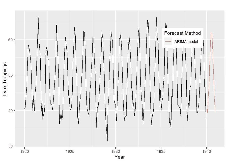
Grafikte model mevsimsel döngüyü yakalıyor: yaz tepeleri ve kış dipleri doğru dönemlerde çıkıyor. Ancak tahmin ufku uzadıkça öngörüler serinin ortalamasına doğru yaklaşıyor ve genlik hafifçe sönüyor. Bu bir hata değil, ARIMA'nın doğal davranışı — uzak gelecek için model, elindeki bilgiyi tükettiğinde ortalamaya yakınsar.
Pratik sonuç: ARIMA kısa vadede güçlü, uzun vadede temkinli okunmalı. forecast() çıktısındaki tahmin aralıkları da tam olarak bunu gösterir; ufuk uzadıkça bantlar genişler.
11. Sık Yapılan Hatalar
| Hata | Neden problem? | Daha iyi yaklaşım |
|---|---|---|
| Durağanlığı kontrol etmeden modellemek | Sahte regresyon ve güvenilmez katsayılar üretir. | Grafik + korelogram + ADF testini birlikte kullanmak. |
| Gereğinden fazla fark almak | Gürültü artar, model kötüleşir. | En küçük d ile yetinmek; ndiffs() ile kontrol etmek. |
| Mevsimselliği göz ardı etmek | Düzenli örüntü hatada kalır, tahmin sapar. | Frekansı doğru tanımlamak ve mevsimsel terimleri denemek. |
| Farklı veriyle kurulmuş AIC'leri karşılaştırmak | Karşılaştırma geçersizdir. | Aynı gözlem kümesi veya örneklem dışı hata kullanmak. |
auto.arima() çıktısını sorgusuz kabul etmek | Fonksiyon bir arama yapar, bağlamı bilmez. | Artıkları checkresiduals() ile incelemek. |
| Tüm veriyle eğitip aynı veriyle değerlendirmek | Performans olduğundan iyi görünür. | Seriyi zamana göre eğitim/test diye bölmek. |
Sonuç
Zaman serisi analizi, sırası olan veriyi doğru okumak için ayrı bir disiplin. Akış her zaman benzer: seriyi tanı, bileşenlerine ayır, durağanlığı kontrol et, korelogramlarla mertebeler hakkında fikir edin, modeli kur ve son olarak tahmini hem istatistiksel hem iş bağlamında yorumla.
Buradaki örnekler tek bir veri seti üzerinden ilerledi ama mantık değişmiyor: elektrik talebi, satış adedi, mention hacmi veya web trafiği — hepsinde aynı sorular sorulur. Serinin hangi kısmı trend, hangi kısmı mevsimsellik, geriye ne kaldı ve kalan kısım gerçekten rastlantısal mı?
“İyi bir zaman serisi modeli geleceği bilmez; belirsizliğin ne kadar olduğunu dürüstçe söyler.”
The moment a time stamp is attached to a column of numbers, the problem changes. Observations are no longer independent: today's value depends on yesterday's, and this month's on the same month last year. The “observations are independent” assumption behind classical regression breaks down, and the data calls for its own toolkit.
In this post I work through the core ideas of time series analysis in R: decomposing a series into its components, stationarity, autocorrelation, and forecasting with ARIMA. All examples use nottem, a data set that ships with R, so you can reproduce them without downloading anything.
“The real question in time series analysis is not ‘which model is better?' but ‘which part of this series is systematic and which part is chance?'”
1. What Is a Time Series?
A time series is data formed by ordering observations of a variable by time. With T as the sample size, it is usually written as Xt, t = 1, 2, …, T.
Continuous
Data that can be recorded without interruption: electrical signals, vibration.
Discrete
Data obtained only at specific moments: interest rates, monthly sales volume.
Regular
Equal intervals between observations: daily, monthly, quarterly.
Irregular
Unequal intervals; most methods require regularizing the series first.
In R, what turns a vector into a time series is the ts class and its frequency. Frequency says how many observations make up one seasonal cycle: 12 for monthly data, 4 for quarterly. Every seasonal calculation that follows rests on this single number.
library(tidyverse)
library(forecast)
library(tseries)

# nottem: monthly average air temperature at Nottingham Castle (°F), 1920-1939
class(nottem)      # "ts"
frequency(nottem)  # 12 -> monthly
start(nottem)      # 1920 1

autoplot(nottem) +
  labs(title = "Monthly average temperature in Nottingham",
       x = "Year", y = "Temperature (°F)")
2. The Components of a Series
A time series combines deterministic elements, which can be written as a formula, with stochastic elements that arise from random processes. Classical decomposition reduces this structure to four components.
| Component | Symbol | What it captures |
|---|---|---|
| Trend | T | The long-run upward or downward movement of the series. |
| Seasonality | S | Fluctuation that repeats with a fixed period (months of the year, days of the week). |
| Cycle | C | Waves longer than seasonality with no fixed period; economic cycles. |
| Irregular / random | I | Everything else: the unexplained part. |
These components can combine in two ways. The additive model fits when the amplitude of the seasonal swing is independent of the level of the series:
The multiplicative model is used when the seasonal swing grows along with the level:
3. Decomposition with decompose()
In R, decompose() estimates the trend with moving averages, extracts seasonal averages from the detrended series, and returns what is left as the random component.
parts <- decompose(nottem)        # default: type = "additive"
plot(parts)

# Accessing the components one by one
parts$trend
parts$seasonal
parts$random

# Multiplicative decomposition
plot(decompose(nottem, type = "multiplicative"))The chart has four panels: the observed series, the trend, the seasonal component and the random component. For nottem, the seasonal panel shows a wave that repeats almost exactly, while the trend panel has no clear direction — across 20 years the average temperature moves within a narrow band.
Because the amplitude of the seasonal wave does not grow over the years, the additive model is the right choice for this series. The classic example of multiplicative behaviour is AirPassengers: as passenger numbers rise, the gap between summer and winter grows in absolute terms, so the amplitude depends on the level.
4. Stationarity
In a stationary series the mean, the variance and the covariance at given lags do not change over time. Whatever window you cut the series at, its statistical behaviour is the same.
Why does this matter? Because forecasting rests on the assumption that behaviour observed in the past will continue to hold. In a non-stationary series that assumption fails: the model fits the past but does not carry into the future. On top of that, two non-stationary series can produce a high R² with no real relationship between them at all — a spurious regression.
Stable structure
Mean and variance do not change over time; shocks die out.
Has memory
Each value is the previous one plus a shock; the effect of shocks is permanent.
Structureless
Zero mean, constant variance, no relationship between lags.
The random walk is the best-known example of a non-stationary series:
Here et is white noise. The model itself is not stationary, because every shock is added permanently to the level of the series. The most common way to make a series stationary is differencing: taking the difference between consecutive observations reduces a random walk to white noise.
5. Autocorrelation: ACF and PACF
While correlation measures the linear relationship between two variables, autocorrelation measures the relationship of a series with its own lagged values. rk is the relationship between the series and its k-lagged version:
Plotting these coefficients against the lag gives the correlogram (ACF). The partial autocorrelation (PACF) shows the direct relationship that remains once the effect of the intermediate lags has been removed.
ggAcf(nottem, lag.max = 25) +
  labs(title = "nottem — autocorrelation (ACF)")

ggPacf(nottem, lag.max = 42) +
  labs(title = "nottem — partial autocorrelation (PACF)")
The blue dashed lines are the confidence bounds. When reading these plots, look for:
| What you see | What it means |
|---|---|
| Bars inside the confidence bounds | No significant autocorrelation at that lag. |
| An ACF that starts high and decays very slowly | The series is not stationary; differencing may be needed. |
| Peaks repeating at lags 12, 24, 36… | Seasonality in monthly data. |
| ACF cuts off after lag q | A hint of an MA(q) process. |
| PACF cuts off after lag p | A hint of an AR(p) process. |
6. Unit Roots and the ADF Test
Plots and correlograms give an impression of stationarity but are not enough to decide. The precise measurement comes from unit root tests. In a model where the series is explained by its own lag, the test asks whether the coefficient equals 1:
If ρ = 1 the series has a unit root — it behaves like a random walk and is not stationary. The hypotheses of the Augmented Dickey-Fuller (ADF) test are:
| Hypothesis | Statement |
|---|---|
| H₀ | The series has a unit root (it is not stationary). |
| H₁ | The series has no unit root (it is stationary). |
nottem_random <- decompose(nottem)$random
nottem_random <- na.remove(nottem_random)  # NAs at both ends

tsdisplay(nottem_random)
adf.test(nottem_random) Augmented Dickey-Fuller Test
data: nottem_random
Dickey-Fuller = -8.4454, Lag order = 6, p-value = 0.01
alternative hypothesis: stationaryThe p-value is below 0.05, so H₀ is rejected: once the seasonal and trend components are removed, the series has no unit root and is stationary. We can move on to modelling.
adf.test() in the tseries package computes the p-value from a table and truncates it at the table's limits. The 0.01 here does not mean “exactly 1%” but “smaller than 1%”, and R prints a warning to that effect. Also, stationarity established after decompose() does not mean the raw nottem series is stationary — what was tested is the cleaned series.7. AR, MA and ARMA
There are two basic ways to model a stationary series: explain it with its own past, or explain it with its past errors.
AR(p) — autoregressive process. Today's value is a linear combination of its own lagged values:
MA(q) — moving average process. Today's value is a weighted sum of past error terms:
ARMA(p,q). Most real series show both behaviours; the Box-Jenkins approach combines the two structures:
AR order
How many lagged observations enter the model? The hint is in the PACF.
MA order
How many lagged error terms enter the model? The hint is in the ACF.
Order of differencing
How many times must the series be differenced to become stationary?
8. ARIMA(p,d,q)
ARMA works only on stationary series. For non-stationary series we difference first; adding this integration step, I(d), to the model gives ARIMA(p,d,q). For seasonal series a seasonal group of terms is added as well, and the model is written as ARIMA(p,d,q)(P,D,Q)[m], where m is the frequency.
Orders can also be chosen by hand. Below, three different models are fitted to nottem:
arima(nottem, order = c(2, 0, 0))
arima(nottem, order = c(0, 0, 3))
arima(nottem, order = c(2, 2, 2))| Model | σ² | Log-likelihood | AIC |
|---|---|---|---|
| ARIMA(2,0,0) | 15.87 | −673.30 | 1354.60 |
| ARIMA(0,0,3) | 17.55 | −685.27 | 1380.54 |
| ARIMA(2,2,2) | 25.23 | −721.98 | 1453.96 |
Of the three, ARIMA(2,0,0) has the lowest AIC. The logic is this: AIC accounts for both the fit to the data and the number of parameters, which keeps you out of the “a more complex model is always better” trap.
That ARIMA(2,2,2) performs worst is instructive too. nottem carries no non-stationary trend; differencing it twice adds unnecessary noise instead of fixing anything. Overdifferencing is a common mistake.
9. Choosing a Model with auto.arima()
When the number of series grows, or the data is too large to inspect by eye, trying orders one by one is not practical. auto.arima() from the forecast package determines d and D with unit root tests, then searches over p, q, P and Q using an information criterion.
auto.arima(nottem)

# To see the models that were tried
auto.arima(nottem, trace = TRUE)

# To turn off the stepwise search and search exhaustively
auto.arima(nottem, trace = TRUE, stepwise = FALSE)Series: nottem
ARIMA(1,0,2)(1,1,2)[12] with drift
sigma^2 estimated as 5.22: log likelihood=-516.48
AIC=1048.96 AICc=1049.62 BIC=1076.4None of the models we tried by hand had a seasonal term; auto.arima() added the [12] seasonal component and a seasonal difference of D = 1. The error variance fell from 15.87 to 5.22 — seasonality accounts for most of the explained variation in this series.
With the stepwise search turned off (stepwise = FALSE) every combination of orders is tried and a slightly better model is found: ARIMA(1,0,1)(1,1,2)[12], AIC = 1046.49. The gain is small, while the search takes noticeably longer.
D = 1 and therefore work with 12 fewer observations. Reading 1354.60 against 1048.96 as “twice as good” is therefore wrong. The correct comparison trains the models on the same data and splits the series to measure out-of-sample error (for example, holding out the last 24 months and looking at RMSE/MAE).10. Forecasting and Interpretation
Once a model is fitted, forecast() produces predictions. Below, a 12-month forecast:
model <- auto.arima(nottem)
fc <- forecast(model, h = 12)

autoplot(fc) +
  labs(title = "nottem — 12-month ARIMA forecast",
x = "Year", y = "Temperature (°F)")The model captures the seasonal cycle: summer peaks and winter troughs appear in the right periods. But as the horizon lengthens, the forecasts move towards the mean of the series and the amplitude flattens slightly. This is not a flaw but ARIMA's natural behaviour — for the distant future, once the model has used up the information it has, it converges to the mean.
The practical takeaway: ARIMA is strong in the short run and should be read cautiously in the long run. The prediction intervals in the forecast() output say exactly the same thing; the bands widen as the horizon grows.
11. Common Mistakes
| Mistake | Why it is a problem | A better approach |
|---|---|---|
| Modelling without checking stationarity | Produces spurious regressions and unreliable coefficients. | Use the plot, the correlogram and the ADF test together. |
| Differencing more than necessary | Adds noise and makes the model worse. | Use the smallest d; check with ndiffs(). |
| Ignoring seasonality | A regular pattern is left in the errors and forecasts drift. | Set the frequency correctly and try seasonal terms. |
| Comparing AIC values from different data | The comparison is invalid. | Use the same set of observations, or out-of-sample error. |
Accepting auto.arima() without question | The function runs a search; it does not know the context. | Inspect the residuals with checkresiduals(). |
| Training and evaluating on all the data | Performance looks better than it is. | Split the series into training and test by time. |
Conclusion
Time series analysis is a separate discipline for reading data that has an order. The flow is always similar: get to know the series, decompose it, check stationarity, use the correlograms to form an idea about the orders, fit the model, and finally interpret the forecast both statistically and in business terms.
The examples here ran on a single data set, but the logic does not change: electricity demand, units sold, mention volume or web traffic — the same questions apply to all of them. Which part of the series is trend, which part is seasonality, what is left over, and is what is left really random?
“A good time series model does not know the future; it is honest about how much uncertainty there is.”