
Varyans Enflasyon Faktörü (VIF) ve Çoklu Doğrusal Bağlantı
VIF = 1/(1−R²) formülünün arkasında ne var? Değerleri standart hata çarpanına çevirmeyi, korelasyon matrisinin neden yetmediğini ve yüksek VIF'te değişken atmanın neden çoğu zaman yanlış cevap olduğunu anlatıyorum.
- İstatistik
- Makine Öğrenmesi
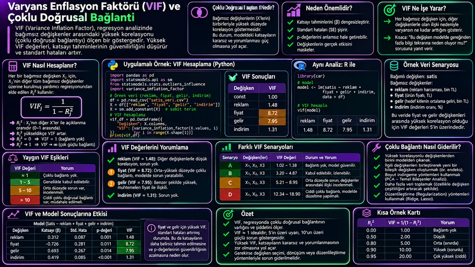
Çoklu doğrusal bağlantı nedir?
Çoklu doğrusal bağlantı (multicollinearity), regresyondaki açıklayıcı değişkenlerden birinin diğerleriyle doğrusal olarak açıklanabilmesidir. En uç örnek bir uzunluğu hem santimetre hem metre cinsinden modele koymaktır: iki sütun birbirinin tam katıdır. Pratikte daha sık karşılaşılan hâli daha yumuşaktır — gelir ve harcama, ziyaretçi sayısı ve oturum sayısı, mağaza büyüklüğü ve çalışan sayısı gibi birbirine yakın kavramlar.
Bağlantı arttıkça model, her değişkenin sonuca ayrı katkısını ayırt etmekte zorlanır. Sonuç olarak katsayı standart hataları büyür, güven aralıkları genişler, p-değerleri yükselir ve örneklem biraz değiştiğinde katsayılar oynar — hatta işaret değiştirebilir.
VIF neyi ölçer?
VIF'in mantığı şaşırtıcı derecede basittir. Her açıklayıcı değişken için, o değişkeni diğer açıklayıcı değişkenlerle tahmin eden bir yardımcı regresyon kurarsınız. Bu yardımcı modelin belirleme katsayısı R²j olsun. O zaman:
Buradaki R²j, ana modelin değil, j değişkeninin diğer açıklayıcılarla tahmin edildiği yardımcı modelin R-karesidir. Hedef değişken bu hesaba hiç girmez.
Formülün söylediği şu: j değişkeni diğerleri tarafından ne kadar iyi açıklanıyorsa, VIF o kadar büyür. R² = 0 ise VIF = 1, yani hiç örtüşme yok. R² = 0,9 ise VIF = 10.
VIF'in adındaki "varyans şişirme" ifadesi birebir doğrudur: katsayı tahmininin varyansı, hiç bağlantı olmayan duruma göre VIF katı büyümüştür. Standart hata varyansın karekökü olduğu için, standart hatadaki artış yaklaşık √VIF katıdır. Pratikte işinize yarayacak sayı budur.
Değerleri somutlaştıralım
| VIF | Yardımcı R² | Varyans çarpanı | Standart hata çarpanı | Yorum |
|---|---|---|---|---|
| 1,0 | %0 | 1 kat | 1 kat | Doğrusal örtüşme yok. |
| 2,5 | %60 | 2,5 kat | 1,58 kat | Bir miktar örtüşme; çoğu uygulamada sorun değil. |
| 5,0 | %80 | 5 kat | 2,24 kat | Güven aralığı iki katına çıktı; sebebini araştırın. |
| 10,0 | %90 | 10 kat | 3,16 kat | Ayrı katsayı yorumu kırılgan hâle gelir. |
| ∞ / çok büyük | ≈%100 | Hesaplanamaz | Hesaplanamaz | Tam veya neredeyse tam doğrusal bağımlılık var. |
Tabloyu "standart hata çarpanı" sütunundan okuyun. VIF = 10 demek, o katsayının güven aralığının bağlantısız duruma göre yaklaşık üç kat geniş olması demektir. Anlamlı çıkmayan bir katsayı, gerçekten etkisiz olduğu için değil, basitçe ölçemediğiniz için anlamsız çıkmış olabilir.
Korelasyon matrisi neden yetmez?
Akla gelen ilk yöntem korelasyon matrisine bakmaktır ve bu yararlıdır — ama eksiktir. Pearson korelasyonu yalnızca ikili ilişkiyi ölçer. Oysa bir değişken, tek tek hiçbiriyle güçlü korelasyon göstermediği hâlde, birkaç değişkenin birleşimiyle neredeyse mükemmel açıklanabilir.
Klasik örnek: modelde "toplam gelir", "ürün A geliri" ve "ürün B geliri" sütunları birlikte bulunsun. Toplam = A + B olduğu için tam bir doğrusal bağımlılık vardır, ama toplam ile A arasındaki ikili korelasyon 0,7 gibi masum bir değer olabilir. Korelasyon matrisi bunu kaçırır; VIF kaçırmaz.
Öte yandan VIF de her şeyi söylemez: ilişkinin yönünü, değişkenlerin kavramsal olarak birbirinin yerine geçip geçemeyeceğini ve modelin tahmin kalitesini göstermez. Korelasyon tablosu, saçılım grafikleri ve alan bilgisiyle birlikte okuyun.
Python ile VIF hesaplama
statsmodels, tasarım matrisini ve hesaplanacak sütunun indeksini ister. Formula arayüzü kullanıyorsanız sabit terim de matriste yer alır; sabit terimin VIF'ini yorumlamayın, o yalnızca ortalamaların merkezlenmesiyle ilgilidir.
import pandas as pd
import statsmodels.formula.api as smf
from statsmodels.stats.outliers_influence import variance_inflation_factor

model = smf.ols(
    "satis ~ reklam + fiyat + ziyaretci + web_oturumu",
    data=df
).fit()

X = model.model.exog
isimler = model.model.exog_names

vif = pd.DataFrame({
    "degisken": isimler,
    "VIF": [variance_inflation_factor(X, i)
            for i in range(X.shape[1])],
})

print(vif[vif["degisken"] != "Intercept"].round(2))
Kategorik değişkenleri dummy kodlamayla modele aldıysanız dikkat: her dummy sütunu için ayrı bir VIF çıkar ve bunlar doğal olarak birbirine bağlıdır. Çok kategorili bir değişkende yüksek VIF görmek tek başına sorun işareti olmayabilir; bu durumda değişken grubu için genelleştirilmiş VIF (GVIF) daha uygun bir ölçüdür.
Bir tabloyu adım adım okuyalım
Bir satış modelinde VIF tablosu şöyle çıksın:
| Değişken | VIF | Yardımcı R² | SE çarpanı | Değerlendirme |
|---|---|---|---|---|
| Reklam harcaması | 1,4 | %29 | 1,18 | Diğerlerinden büyük ölçüde ayrışıyor. |
| Mağaza büyüklüğü | 2,2 | %55 | 1,48 | Hafif örtüşme; sorun değil. |
| Ziyaretçi sayısı | 6,3 | %84 | 2,51 | Belirgin örtüşme, incelenmeli. |
| Web oturumu | 9,1 | %89 | 3,02 | Ziyaretçi sayısıyla neredeyse aynı bilgiyi taşıyor. |
Web oturumu için hesabı açalım: VIF = 9,1 ise yardımcı regresyonda R² = 1 − 1/9,1 = 0,89. Yani diğer açıklayıcı değişkenler, web oturumu değişkenliğinin yaklaşık %89'unu doğrusal olarak açıklıyor. Standart hata, bağlantısız duruma göre √9,1 ≈ 3 kat geniş.
Buradan çıkarılacak doğru sonuç şu değildir: "web oturumunu modelden at." Doğru sonuç şudur: ziyaretçi sayısı ile web oturumu aynı olguyu iki farklı şekilde ölçüyor olabilir; bu iki katsayıyı ayrı ayrı yorumlamak güvenilir değil. Karar, istatistikten değil alan bilgisinden gelir — bu iki metrik iş açısından farklı şeyler mi ölçüyor?
Eşikler kural değil, uyarıdır
Literatürde 5 ve 10 eşikleri sık geçer, ama bunlar istatistiksel olarak türetilmiş sınırlar değildir; pratikten gelen kaba işaretlerdir. Bir eşiği mekanik olarak uygulamak iki yönde de hata üretir.
Düşük VIF modelin doğru kurulduğunu göstermez — eksik değişken, yanlış fonksiyonel biçim veya endojenlik sorunları VIF'e hiç yansımaz. Yüksek VIF de modeli kullanılamaz yapmaz. Asıl soru şudur: bu katsayıyı ne için kullanacağım?
| Amacınız | Yüksek VIF ne kadar önemli? | Neden? |
|---|---|---|
| Tahmin yapmak | Çoğu zaman önemsiz | Birlikte hareket eden değişkenler tahmin gücünü bozmaz. |
| Tek bir değişkenin etkisini yorumlamak | Çok önemli | O katsayının belirsizliği doğrudan şişer. |
| Değişken önemini sıralamak | Önemli | Sıralama örneklemden örnekleme değişebilir. |
| Model karşılaştırmak | Dolaylı | Çapraz doğrulama hatası daha doğrudan bir ölçüttür. |
Yüksek VIF görünce ne yapmalı?
- Matrisi
Kontrol Et - Alan Anlamını
İncele - Gerekçeli
Seçim Yap - Özet Ölçü
veya Ridge - Etkiyi
Raporla
- Önce yapısal hata arayın. Aynı değişken iki kez mi eklendi? Toplam ve bileşenleri birlikte mi duruyor? Dummy değişkenlerin hepsi mi modelde (dummy-variable trap)? Bu tür hatalar VIF'i yapay olarak uçurur ve düzeltilmesi en kolay olanlardır.
- Alan anlamına bakın. İki değişken aynı olguyu mu ölçüyor, yoksa farklı mekanizmaları mı temsil ediyor? "Ziyaretçi sayısı" ile "web oturumu" aynıya yakınken, "reklam harcaması" ile "mağaza büyüklüğü" farklı şeylerdir.
- Gerekçeli seçim yapın. Benzer iki göstergeden biri ölçüm kalitesi, veri bulunurluğu veya iş sorusuna uygunluk bakımından öne çıkıyorsa onu tutun ve kararı yazın.
- Özet ölçü veya düzenlileştirme düşünün. Birkaç benzer gösterge açıkça tanımlanmış bir endekse dönüştürülebilir. Amaç tahminse Ridge regresyon, bağlantılı katsayıları küçülterek kararlılık sağlar — ama katsayı yorumu OLS'ten farklılaşır.
- Etkiyi raporlayın. Değişikliğin öncesi ve sonrasında katsayıları, standart hataları ve tahmin performansını yan yana gösterin.
Bir not daha: etkileşim ve polinom terimlerinde merkezleme (değişkenden ortalamasını çıkarma) yapay sayısal bağlantıyı azaltabilir. Bu gerçek bir bilgi örtüşmesini ortadan kaldırmaz, yalnızca ölçekten kaynaklanan kısmı temizler.
VIF'in sınırları
Hedefi görmez
VIF yalnızca açıklayıcı tasarım matrisine bakar; bağımlı değişken hesaba hiç girmez.
Yön söylemez
Hangi değişkenin hangisini açıkladığını veya nedensellik yönünü belirtmez.
Yalnızca doğrusal
Doğrusal olmayan bağımlılıkları yakalamaz. İki değişken eğrisel olarak bağlı olsa da VIF düşük çıkabilir.
Dummy'lerde karışır
Çok kategorili değişkenlerde sütun bazlı VIF yanıltıcıdır; GVIF daha uygundur.
Ölçekten etkilenir
Etkileşim ve polinom terimlerinde merkezleme yapmadan okunan VIF şişmiş görünebilir.
Eşik evrensel değil
5 ve 10 sayıları gelenektir; alana, örneklem büyüklüğüne ve amaca göre değişir.
Kontrol listesi
- Tasarım matrisinde yapısal bir tekrar veya toplam-bileşen çakışması var mı?
- VIF her açıklayıcı sütun için hesaplandı mı, sabit terim dışlandı mı?
- Yüksek değerler yardımcı R² ve √VIF cinsinden yorumlandı mı?
- Korelasyon matrisi ve saçılım grafikleri de incelendi mi?
- Katsayı standart hataları ve güven aralıkları gözden geçirildi mi?
- Değişken çıkarma kararı alan bilgisiyle gerekçelendirildi mi?
- Amacın tahmin mi yoksa çıkarım mı olduğu netleştirildi mi?
- Yapılan değişikliğin katsayılara etkisi öncesi/sonrası raporlandı mı?
Sonuç
VIF, bir katsayının ne kadar güvenilir ölçülebildiğini gösteren bir tanı aracıdır — geçilmesi gereken bir sınav değil. Sayıyı tek başına bir eşikle karşılaştırmak yerine, √VIF üzerinden "bu katsayının güven aralığı kaç kat genişledi?" sorusuna çevirin. O zaman sayı anlam kazanır.
Ve asıl soruyu unutmayın: bu modeli tahmin için mi, yoksa tek tek değişkenlerin etkisini yorumlamak için mi kuruyorsunuz? Cevap, yüksek bir VIF'in ciddi bir sorun mu yoksa dipnot mu olduğunu belirler.
What is multicollinearity?
Multicollinearity means that one of the explanatory variables in a regression can be explained linearly by the others. The extreme example is putting the same length into the model in both centimetres and metres: one column is an exact multiple of the other. In practice you meet softer versions far more often — income and spending, visitor count and session count, store size and headcount.
As collinearity rises, the model struggles to separate each variable's individual contribution to the outcome. Coefficient standard errors grow, confidence intervals widen, p-values rise, and the coefficients move around when the sample changes slightly — they can even flip sign.
What does VIF measure?
The logic of VIF is surprisingly simple. For each explanatory variable, you fit an auxiliary regression that predicts it from the other explanatory variables. Let the coefficient of determination of that auxiliary model be R²j. Then:
That R²j belongs to the auxiliary model in which variable j is predicted from the other explanatory variables, not to the main model. The target variable never enters this calculation.
What the formula says: the better variable j is explained by the others, the larger VIF gets. R² = 0 gives VIF = 1, meaning no overlap at all. R² = 0.9 gives VIF = 10.
The "variance inflation" in the name is literal: the variance of the coefficient estimate is VIF times what it would be with no collinearity. Because the standard error is the square root of the variance, the increase in the standard error is roughly √VIF. That is the number you will actually use.
Making the values concrete
| VIF | Auxiliary R² | Variance factor | Std. error factor | Reading |
|---|---|---|---|---|
| 1.0 | 0% | 1× | 1× | No linear overlap. |
| 2.5 | 60% | 2.5× | 1.58× | Some overlap; fine in most applications. |
| 5.0 | 80% | 5× | 2.24× | The confidence interval doubled; find out why. |
| 10.0 | 90% | 10× | 3.16× | Interpreting that coefficient alone becomes fragile. |
| ∞ / very large | ≈100% | Undefined | Undefined | Exact or near-exact linear dependence. |
Read the table from the "standard error factor" column. VIF = 10 means that coefficient's confidence interval is about three times wider than it would be without collinearity. A coefficient that comes out non-significant may be so not because it has no effect, but simply because you could not measure it.
Why isn't a correlation matrix enough?
The first method that comes to mind is to look at the correlation matrix, and that is useful — but incomplete. Pearson correlation measures only the pairwise relationship. A variable can show no strong correlation with any single other variable and still be explained almost perfectly by a combination of several.
The classic example: the model contains "total revenue", "product A revenue" and "product B revenue" together. Because total = A + B there is an exact linear dependence, yet the pairwise correlation between total and A might be an innocent-looking 0.7. The correlation matrix misses this; VIF does not.
On the other hand, VIF does not tell you everything either: not the direction of the relationship, not whether two variables are conceptually interchangeable, and not the model's predictive quality. Read it alongside the correlation table, scatter plots and domain knowledge.
Computing VIF in Python
statsmodels wants the design matrix and the index of the column to compute. If you use the formula interface, the intercept is part of that matrix; do not interpret the intercept's VIF — it only reflects the centring of the means.
import pandas as pd
import statsmodels.formula.api as smf
from statsmodels.stats.outliers_influence import variance_inflation_factor

model = smf.ols(
    "sales ~ adspend + price + visitors + web_sessions",
    data=df
).fit()

X = model.model.exog
names = model.model.exog_names

vif = pd.DataFrame({
    "variable": names,
    "VIF": [variance_inflation_factor(X, i)
            for i in range(X.shape[1])],
})

print(vif[vif["variable"] != "Intercept"].round(2))
Be careful with categorical variables entered as dummies: you get a separate VIF for each dummy column, and those are naturally linked to one another. A high VIF on a many-level categorical variable is not by itself a warning sign; a generalised VIF (GVIF) for the variable group is the more appropriate measure there.
Reading a table step by step
Suppose a sales model produces this VIF table:
| Variable | VIF | Auxiliary R² | SE factor | Assessment |
|---|---|---|---|---|
| Ad spend | 1.4 | 29% | 1.18 | Largely distinct from the others. |
| Store size | 2.2 | 55% | 1.48 | Mild overlap; not a problem. |
| Visitor count | 6.3 | 84% | 2.51 | Clear overlap, worth examining. |
| Web sessions | 9.1 | 89% | 3.02 | Carries almost the same information as visitors. |
Let us work web sessions out: with VIF = 9.1, the auxiliary R² is 1 − 1/9.1 = 0.89. The other explanatory variables explain roughly 89% of the variation in web sessions linearly. Its standard error is about √9.1 ≈ 3 times wider than it would be without collinearity.
The right conclusion is not "drop web sessions from the model". It is this: visitor count and web sessions may be measuring the same phenomenon two different ways, so interpreting those two coefficients separately is not reliable. The decision comes from domain knowledge, not from statistics — do these two metrics measure different things in business terms?
Thresholds are warnings, not rules
Thresholds of 5 and 10 appear often in the literature, but they are not statistically derived boundaries; they are rough signals drawn from practice. Applying one mechanically produces errors in both directions.
A low VIF does not show the model is correctly specified — omitted variables, the wrong functional form and endogeneity never show up in VIF at all. A high VIF does not make a model unusable either. The real question is: what am I going to use this coefficient for?
| Your goal | How much does high VIF matter? | Why? |
|---|---|---|
| Making predictions | Usually not much | Variables that move together do not hurt predictive power. |
| Interpreting one variable's effect | A great deal | The uncertainty on that coefficient inflates directly. |
| Ranking variable importance | Considerably | The ranking can change from sample to sample. |
| Comparing models | Indirectly | Cross-validated error is a more direct criterion. |
What to do when VIF is high
- Check the
Matrix - Examine the
Domain - Make a
Reasoned Choice - Index or
Ridge - Report the
Effect
- Look for a structural mistake first. Was the same variable added twice? Are a total and its components both in the model? Are all dummy levels present (the dummy-variable trap)? Errors like these inflate VIF artificially and are the easiest to fix.
- Look at the domain meaning. Do the two variables measure the same phenomenon, or do they represent different mechanisms? "Visitor count" and "web sessions" are near-duplicates; "ad spend" and "store size" are not.
- Make a reasoned choice. If one of two similar indicators stands out on measurement quality, data availability or fit with the business question, keep it and write the decision down.
- Consider a summary measure or regularisation. Several similar indicators can be turned into a clearly defined index. If the goal is prediction, ridge regression shrinks correlated coefficients and buys stability — though coefficient interpretation then differs from OLS.
- Report the effect. Show coefficients, standard errors and predictive performance before and after the change, side by side.
One more note: for interaction and polynomial terms, centring (subtracting the mean) can reduce artificial numerical collinearity. It does not remove a real overlap in information, only the part that comes from scale.
The limits of VIF
It ignores the target
VIF looks only at the explanatory design matrix; the dependent variable never enters.
No direction
It does not say which variable explains which, or anything about causality.
Linear only
It does not catch non-linear dependence. Two variables can be curvilinearly related with a low VIF.
Dummies confuse it
Column-wise VIF is misleading for many-level categoricals; GVIF fits better.
Scale affects it
Read without centring, VIF on interaction and polynomial terms can look inflated.
No universal cutoff
The numbers 5 and 10 are convention; they shift with the field, the sample size and the goal.
Checklist
- Is there a structural duplicate or a total-and-components clash in the design matrix?
- Was VIF computed for every explanatory column, with the intercept excluded?
- Were high values read in terms of auxiliary R² and √VIF?
- Were the correlation matrix and scatter plots examined too?
- Were coefficient standard errors and confidence intervals reviewed?
- Was any decision to drop a variable justified with domain knowledge?
- Is it clear whether the goal is prediction or inference?
- Was the before/after effect on the coefficients reported?
Conclusion
VIF is a diagnostic that shows how reliably a coefficient can be measured — not an exam to be passed. Rather than comparing the number to a threshold, translate it through √VIF into "how many times wider did this coefficient's confidence interval get?". That is when the number starts to mean something.
And do not lose sight of the real question: are you building this model to predict, or to interpret the effect of individual variables? The answer determines whether a high VIF is a serious problem or a footnote.