R Markdown Nedir? Analizleri Raporlama ve Otomatikleştirme
Kodu, metni ve çıktıyı tek kaynakta birleştiren R Markdown ile tekrarlanabilir rapor üretmeyi; chunk seçenekleri, parametreler ve otomasyonla birlikte ele alıyorum.
- Araçlar
Kod bir dosyada, grafikler bir klasörde, bulgular ise sonradan elle doldurulan bir Word belgesinde. Periyodik raporlarla çalışan herkesin tanıdığı bir dağınıklık bu ve asıl maliyeti analizi ilk kez yapmak değil, aynı süreci her ay yeniden yürütmek.
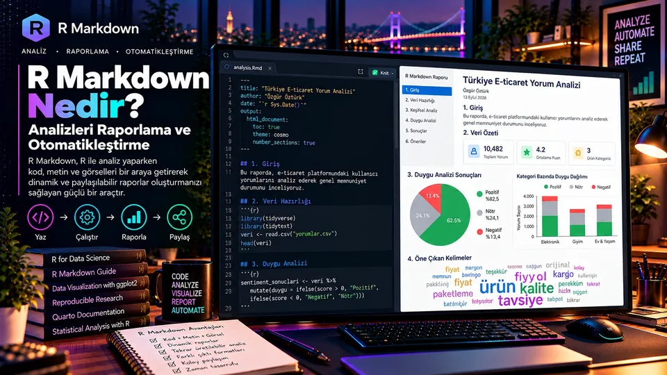
R Markdown, analiz kodunu, açıklayıcı metni ve üretilen çıktıları tek bir rapor kaynağında birleştiren bir raporlama yaklaşımı. Bir .Rmd dosyası; Markdown ile yazılmış metin, R kod blokları ve belgenin nasıl üretileceğini belirleyen YAML üst bilgisinden oluşuyor. Dosya işlendiğinde kod çalışıyor, tablolar ve grafikler oluşuyor, sonuçlar açıklamalarla birlikte seçilen formata yerleşiyor.
“R Markdown yalnızca grafikleri bir belgeye koymaz; o grafiklerin nasıl üretildiğini de raporun kaynağında tutar.”
1. Raporu Otomatikleştirmenin Gerçek Faydası
Veri yenilendiğinde tabloyu yeniden kopyalamak, grafikleri dışa aktarmak ve açıklamaları elle güncellemek hem zaman kaybettirir hem de eski bir değerin raporda kalması gibi sessiz hatalara kapı açar. Tek kaynaklı bir rapor bu adımları ortadan kaldırır.
Rapor üretimi
Aynı şablon ve analiz adımları, dönemler arası karşılaştırmayı tutarlı kılar. Başlık, metrik tanımı ve grafik biçimi her raporda korunur.
Analiz ile yorum
Bir sonuç değiştiğinde onu üreten kod aynı kaynakta görünür; bulgunun hangi veri ve işlemden geldiği izlenebilir.
Paydaşa uygun
Teknik kod ile yönetici özeti aynı belgede birleşebilir; gerekirse kod çıktıda gizlenir.
Düşük maliyet
Yeni dönem için dosya kopyalamak yerine veri ve parametre güncellenip aynı şablon yeniden çalıştırılır.
2. Bir .Rmd Dosyasının Anatomisi
Bir R Markdown dosyası üç katmandan oluşur: YAML üst bilgisi belge ayarlarını, Markdown metni açıklamaları, kod blokları ise hesaplamaları tanımlar.
---
title: "Aylık Satış Performansı"
author: "Veri Analizi Ekibi"
date: "`r Sys.Date()`"
output:
  html_document:
    toc: true
    toc_float: true
    theme: readable
---

# Yönetici Özeti

Bu rapor, seçilen dönemdeki satış performansını inceler.

```{r setup, include=FALSE}
knitr::opts_chunk$set(
  echo = FALSE,
  warning = FALSE,
  message = FALSE
)
```

## Veri ve Yöntem

Aşağıdaki analiz, kategori bazında geliri özetler.| Parça | Rolü | Pratik not |
|---|---|---|
| YAML | Başlık, yazar, tarih ve çıktı biçimi | Dosyanın en başına, iki adet üç-tire satırı arasına yazılır. |
| Markdown | Başlıklar, listeler, bağlantılar ve anlatı | Yöntemin ve bağlamın yazıldığı yer burasıdır. |
| R chunk | Kodu çalıştırıp sonucu belgeye ekler | Chunk'lara anlamlı isim vermek bakımı kolaylaştırır. |
İş bölümü şöyle: knitr kod bloklarını işler, rmarkdown ise belgeyi HTML, PDF veya Word'e dönüştüren render sürecini yönetir.
3. Chunk Seçenekleri: Kod Ne Zaman Çalışsın, Ne Görünsün?
Bir raporda her kod satırının görünmesi gerekmez. Chunk seçenekleri sunum biçimini değiştirir; kodun analiz mantığını değil.
```{r category-summary, echo=FALSE, message=FALSE, warning=FALSE}
summary_table <- sales |>
  dplyr::group_by(category) |>
  dplyr::summarise(revenue = sum(revenue), .groups = "drop")

knitr::kable(summary_table)
```| Seçenek | Ne yapar? | Dikkat |
|---|---|---|
echo=FALSE | Kodu gizler, çıktıyı gösterir. | Teknik olmayan okuyucuya yönelik raporlarda yararlıdır. |
include=FALSE | Kodu çalıştırır, ne kodu ne çıktıyı rapora ekler. | Veri hazırlama ve kurulum ayarları için uygundur. |
eval=FALSE | Kodu gösterir ama çalıştırmaz. | Çalıştırılması istenmeyen eğitim örnekleri için. |
message=FALSE | Paket ve işlem mesajlarını gizler. | Gerçek hataları gizlemek için kullanılmamalı. |
warning=FALSE | Uyarıları çıktıda göstermez. | Uyarıyı anlamadan kapatmak sorunları görünmez kılar. |
cache=TRUE | Chunk çıktısını önbelleğe alır. | Veri veya bağımlılık değiştiğinde önbelleğin geçerliliği kontrol edilmeli. |
warning=FALSE ve message=FALSE kodun sorunsuz çalıştığını kanıtlamaz. Geliştirme sırasında uyarıları incelemek, son rapordan önce ise temiz bir oturumda render testi yapmak daha güvenli.4. Uçtan Uca Örnek: Satış Verisinden Rapora
Aşağıdaki örnek küçük bir satış veri seti hazırlıyor, kategori bazında geliri hesaplıyor ve sonucu tabloyla grafiğe dönüştürüyor. Gerçek bir projede aynı yapıya CSV, Excel veya veri tabanı kaynağı bağlanabilir.
```{r sales-summary, message=FALSE}
library(dplyr)
library(ggplot2)
library(knitr)

sales <- data.frame(
  date = as.Date(c(
    "2026-01-05", "2026-01-12", "2026-02-03",
    "2026-02-17", "2026-03-01", "2026-03-11"
  )),
  category = c(
    "Elektronik", "Ev", "Elektronik",
    "Giyim", "Ev", "Giyim"
  ),
  revenue = c(4200, 1800, 2600, 950, 2200, 1500)
)

category_summary <- sales |>
  group_by(category) |>
  summarise(
    total_revenue = sum(revenue),
    transaction_count = n(),
    .groups = "drop"
  ) |>
  arrange(desc(total_revenue))

knitr::kable(
  category_summary,
  caption = "Kategori Bazında Gelir Özeti",
  col.names = c("Kategori", "Toplam gelir", "İşlem sayısı")
)
```
Özet tablosu hesaplandıktan sonra aynı nesne kullanılarak grafik hazırlanabilir:
```{r category-chart, fig.width=8, fig.height=4}
ggplot(
  category_summary,
  aes(x = reorder(category, total_revenue), y = total_revenue)
) +
  geom_col(fill = "#8B7CFF", width = 0.68) +
  coord_flip() +
  scale_y_continuous(
    labels = scales::label_number(big.mark = ".", decimal.mark = ",")
  ) +
  labs(title = "Kategori Bazında Toplam Gelir", x = NULL, y = "Gelir") +
  theme_minimal(base_size = 12)
```category_summary nesnesinden üretiliyor. Hesaplama mantığı iki ayrı yere kopyalanmadığı için sonuçlar arasında tutarsızlık oluşma ihtimali azalıyor.Üretim ortamında bir adım daha gerekir: veri doğrulama. Beklenen kolonlar var mı, tarih aralığı doğru mu, gelir alanında eksik veya negatif değer bulunuyor mu? Rapor yalnızca sayı üretmemeli, verinin beklenen yapıda olduğunu da doğrulamalı.
5. Parametreli Raporlama
Parametreler, aynı şablonun farklı dönemler, bölgeler veya segmentler için kullanılmasını sağlar. Her bölge için ayrı dosya kopyalamak yerine raporun parametresi değişir ve aynı mantıkla yeni çıktı alınır.
---
title: "Bölgesel Satış Raporu"
output: html_document
params:
  selected_region: "Marmara"
  report_year: 2026
---filtered_sales <- sales |>
dplyr::filter(
region == params$selected_region,
format(date, "%Y") == as.character(params$report_year)
)
summary(filtered_sales)Parametre kullanırken değerin veri tipi önemli: yıl parametresi sayısal mı, karakter mi? Yukarıdaki örnekte as.character() tam olarak bu belirsizliği kapatmak için var. Filtre sonrası hiç kayıt kalmaması durumu da ele alınmalı.
6. Raporları Otomatik Üretmek
Rapor üretimini otomatikleştirmek için rmarkdown::render() kullanılır. Bu fonksiyon bir R betiğinden, zamanlanmış görevden veya başka bir iş akışından çağrılabilir.
- Veri alCSV / Excel / DB
- Kontrol etŞema ve kalite
- Analiz etHesaplar ve grafikler
- Render etHTML / PDF / Word
- PaylaşKontrollü dağıtım
rmarkdown::render(
  input = "monthly-report.Rmd",
  output_format = "html_document",
  output_file = "monthly-report.html",
  params = list(
    selected_region = "Marmara",
    report_year = 2026
  ),
  envir = new.env(parent = globalenv())
)
Buradaki envir = new.env(...) küçük ama kritik: raporu temiz bir ortamda çalıştırarak, o anda bellekte duran nesnelere farkında olmadan bağımlı kalmayı önler.
7. Raporun Yeniden Üretilebilir Olması
Veriyi tanımla
Dosya yolu, dönem ve veri kaynağı raporda izlenebilir olsun.
Sabitle
Simülasyon veya örnekleme varsa uygun yerde set.seed() kullan.
Bağımlılıkları izle
Paketlerin başka bir bilgisayarda da kurulabilmesini düşün.
Temiz render
Bellekte duran nesnelere farkında olmadan bağımlı kalma.
Doğrulama ekle
Beklenen satır sayısı, kolon isimleri ve eksik değerler kontrol edilsin.
Çıktıyı incele
Tarih, sayılar, grafikler ve hassas bilgiler paylaşımdan önce gözden geçirilsin.
Tekrar üretilebilirlik yalnızca aynı kodu saklamak değil. Verinin hangi sürümünün kullanıldığı, kodun hangi koşullarda çalıştığı ve sonucu yeniden oluşturmak için hangi bağımlılıkların gerektiği de bu tanımın parçası.
8. R Markdown mı, Quarto mu?
R Markdown uzun süredir kullanılan ve mevcut projelerde sıkça karşılaşılan bir yaklaşım. Quarto ise çok dilli doküman, rapor, sunum ve web yayınları için daha yeni bir yayınlama sistemi. İkisi de tekrarlanabilir raporlama akışı kurar; seçim mevcut proje yapısına göre yapılmalı.
| Kriter | R Markdown | Quarto |
|---|---|---|
| Mevcut R projeleri | Yerleşik bir akış varsa devam etmek pratiktir. | Geçiş yapılacaksa doküman ve çıktı uyumluluğu test edilmeli. |
| Yeni projeler | Özel gereksinimlerde uygun bir seçenek olabilir. | Çok formatlı ve çok dilli yayın akışları için değerlendirmeye değer. |
| Temel yaklaşım | Markdown + kod chunk'ları + render. | Markdown temelli yayın sistemi; birden fazla dil ve çıktı türü. |
9. Kaliteli Bir Rapor İçin Kontrol Listesi
İş sorusu belli
Rapor okuyucunun hangi kararını destekliyor?
Yöntem anlatılmış
Metrik ve filtre tanımları açık mı?
Kod düzenli
Chunk isimleri anlaşılır ve tekrar az mı?
Veri kontrolü var
Eksik veya olağan dışı veriler tespit ediliyor mu?
Çıktı okunabilir
Başlıklar, tablolar, renkler ve sayı biçimleri tutarlı mı?
Otomasyon güvenli
Başarısız üretimde dağıtım engelleniyor mu?
10. Sık Sorulan Sorular
| Soru | Yanıt |
|---|---|
| İleri düzey R bilgisi gerekir mi? | Belge oluşturmak ve basit chunk'lar çalıştırmak için temel R bilgisi yeterli olabilir. Analiz karmaşıklaştıkça veri işleme, hata yönetimi ve kod organizasyonu önem kazanır. |
| PDF üretimi neden hata verir? | PDF çıktısı çoğu akışta LaTeX tabanlı bir araç zinciri gerektirir. HTML çalışırken PDF'in hata vermesi bu yüzden olağandır; ortam ve bağımlılıklar kontrol edilmeli. |
| İnteraktif dashboard oluşturur mu? | R Markdown ağırlıklı olarak rapor üretir. Kullanıcının filtreleri değiştirip sonuçları anlık keşfettiği uygulamalar için R Shiny daha uygun; bazı HTML raporlara ise etkileşimli grafikler eklenebilir. |
Sonuç
R Markdown; kodu, metni ve çıktıyı aynı yerde tutarak veri analizini daha izlenebilir ve sürdürülebilir hale getiriyor. En büyük faydası rapor hazırlamayı hızlandırması değil, rapordaki sonucun hangi veri ve yöntemle üretildiğini görünür kılması.
İyi kurulmuş bir akış; veri doğrulama, analiz, görselleştirme, yorumlama ve render adımlarını birleştirir. Böylece rapor, dönem sonunda hazırlanan bir belge olmaktan çıkıp karar alma sürecinin tekrar üretilebilir bir parçasına dönüşür.
“Analizi bir kez tasarla, raporu güvenilir biçimde yeniden üret.”
The code lives in one file, the charts in a folder, and the findings in a Word document filled in by hand afterwards. Anyone who works with periodic reports knows this mess, and its real cost is not doing the analysis once — it is running the same process again every month.
R Markdown is a reporting approach that brings analysis code, explanatory text and generated output together in a single report source. An .Rmd file consists of text written in Markdown, R code chunks, and a YAML header that defines how the document is produced. When the file is processed, the code runs, tables and charts are generated, and the results land in the chosen output format alongside the narrative.
“R Markdown does not just put charts into a document; it keeps how those charts were produced in the report's source.”
1. The Real Benefit of Automating a Report
When the data refreshes, copying the table again, exporting the charts and updating the commentary by hand costs time and opens the door to quiet errors — such as an old figure left in the report. A single-source report removes those steps.
Report production
The same template and analysis steps make period-to-period comparison consistent. Titles, metric definitions and chart style stay the same.
Analysis and commentary
When a result changes, the code that produced it is visible in the same source; you can trace which data and which operation it came from.
Fit for stakeholders
Technical code and an executive summary can live in one document; the code can be hidden in the output when needed.
Lower cost
Instead of copying a file for the new period, update the data and parameters and re-run the same template.
2. The Anatomy of an .Rmd File
An R Markdown file has three layers: the YAML header defines document settings, the Markdown text carries the narrative, and the code chunks hold the calculations.
---
title: "Monthly Sales Performance"
author: "Data Analytics Team"
date: "`r Sys.Date()`"
output:
  html_document:
    toc: true
    toc_float: true
    theme: readable
---

# Executive Summary

This report reviews sales performance for the selected period.

```{r setup, include=FALSE}
knitr::opts_chunk$set(
  echo = FALSE,
  warning = FALSE,
  message = FALSE
)
```

## Data and Method

The analysis below summarizes revenue by category.| Part | Role | Practical note |
|---|---|---|
| YAML | Title, author, date and output format | Written at the very top, between two lines of three dashes. |
| Markdown | Headings, lists, links and narrative | This is where the method and the context are written. |
| R chunk | Runs code and inserts the result | Giving chunks meaningful names makes maintenance easier. |
The division of labour: knitr processes the code chunks, while rmarkdown manages the render process that converts the document into HTML, PDF or Word.
3. Chunk Options: When Should Code Run, and What Should Show?
Not every line of code needs to appear in a report. Chunk options change how things are presented — not the analysis logic of the code.
```{r category-summary, echo=FALSE, message=FALSE, warning=FALSE}
summary_table <- sales |>
  dplyr::group_by(category) |>
  dplyr::summarise(revenue = sum(revenue), .groups = "drop")

knitr::kable(summary_table)
```| Option | What it does | Watch out for |
|---|---|---|
echo=FALSE | Hides the code, shows the output. | Useful for reports aimed at non-technical readers. |
include=FALSE | Runs the code but adds neither code nor output. | Good for data preparation and setup. |
eval=FALSE | Shows the code but does not run it. | Suitable for teaching examples that should not execute. |
message=FALSE | Hides package and process messages. | Must not be used to hide real errors. |
warning=FALSE | Keeps warnings out of the output. | Silencing a warning you do not understand hides problems. |
cache=TRUE | Caches the chunk output. | Check cache validity when data or dependencies change. |
warning=FALSE and message=FALSE do not prove the code ran cleanly. Review warnings during development, and run a render test in a clean session before the final report.4. End to End: From Sales Data to a Report
The example below prepares a small sales data set, computes revenue by category, and turns the result into a table and a chart. In a real project the same structure can be connected to a CSV, Excel or database source.
```{r sales-summary, message=FALSE}
library(dplyr)
library(ggplot2)
library(knitr)

sales <- data.frame(
  date = as.Date(c(
    "2026-01-05", "2026-01-12", "2026-02-03",
    "2026-02-17", "2026-03-01", "2026-03-11"
  )),
  category = c(
    "Electronics", "Home", "Electronics",
    "Apparel", "Home", "Apparel"
  ),
  revenue = c(4200, 1800, 2600, 950, 2200, 1500)
)

category_summary <- sales |>
  group_by(category) |>
  summarise(
    total_revenue = sum(revenue),
    transaction_count = n(),
    .groups = "drop"
  ) |>
  arrange(desc(total_revenue))

knitr::kable(
  category_summary,
  caption = "Revenue Summary by Category",
  col.names = c("Category", "Total revenue", "Transactions")
)
```
Once the summary table exists, a chart can be built from the same object:
```{r category-chart, fig.width=8, fig.height=4}
ggplot(
  category_summary,
  aes(x = reorder(category, total_revenue), y = total_revenue)
) +
  geom_col(fill = "#8B7CFF", width = 0.68) +
  coord_flip() +
  scale_y_continuous(labels = scales::label_number(big.mark = ",")) +
  labs(title = "Total Revenue by Category", x = NULL, y = "Revenue") +
  theme_minimal(base_size = 12)
```category_summary object. Because the calculation is not copied into two places, the chance of inconsistency between the two drops.In production one more step is needed: data validation. Are the expected columns present, is the date range right, are there missing or negative values in the revenue field? A report should not only produce numbers — it should confirm the data has the expected shape.
5. Parameterized Reporting
Parameters let the same template serve different periods, regions or segments. Instead of copying a file per region, you change the report's parameter and get new output from the same logic.
---
title: "Regional Sales Report"
output: html_document
params:
  selected_region: "Marmara"
  report_year: 2026
---filtered_sales <- sales |>
dplyr::filter(
region == params$selected_region,
format(date, "%Y") == as.character(params$report_year)
)
summary(filtered_sales)The data type of a parameter matters: is the year numeric or character? In the example above, as.character() exists precisely to close that ambiguity. The case where no records remain after filtering must be handled too.
6. Producing Reports Automatically
To automate report production, use rmarkdown::render(). The function can be called from an R script, a scheduled job or another workflow.
- Fetch dataCSV / Excel / DB
- Check itSchema and quality
- AnalyzeCalculations and charts
- RenderHTML / PDF / Word
- ShareControlled distribution
rmarkdown::render(
  input = "monthly-report.Rmd",
  output_format = "html_document",
  output_file = "monthly-report.html",
  params = list(
    selected_region = "Marmara",
    report_year = 2026
  ),
  envir = new.env(parent = globalenv())
)
That envir = new.env(...) is small but critical: it runs the report in a clean environment, preventing an accidental dependency on objects that happen to be in memory.
7. Making the Report Reproducible
Identify the data
File path, period and data source should be traceable in the report.
Fix it
If there is simulation or sampling, use set.seed() in the right place.
Track dependencies
Think about whether the packages can be installed on another machine.
Render clean
Do not depend unknowingly on objects left in memory.
Add validation
Check expected row counts, column names and missing values.
Inspect the output
Dates, numbers, charts and sensitive information should be reviewed before sharing.
Reproducibility is not only about keeping the same code. Which version of the data was used, under what conditions the code ran, and which dependencies are needed to rebuild the result are all part of the definition.
8. R Markdown or Quarto?
R Markdown is a long-established approach you will often meet in existing projects. Quarto is a newer publishing system for multi-language documents, reports, presentations and websites. Both can support a reproducible reporting workflow; the choice depends on the project you already have.
| Criterion | R Markdown | Quarto |
|---|---|---|
| Existing R projects | If a working flow is in place, staying with it is practical. | If you migrate, test document and output compatibility. |
| New projects | Can be the right option for specific requirements. | Worth evaluating for multi-format, multi-language publishing. |
| Core approach | Markdown + code chunks + render. | A Markdown-based publishing system across several languages and output types. |
9. A Checklist for a Quality Report
Clear business question
Which decision does the report support?
Method explained
Are metric and filter definitions stated?
Tidy code
Are chunk names clear and repetition low?
Data checks exist
Are missing or unusual values detected?
Readable output
Are headings, tables, colors and number formats consistent?
Safe automation
Is distribution blocked when a run fails?
10. Frequently Asked Questions
| Question | Answer |
|---|---|
| Do I need advanced R? | Basic R can be enough to create a document and run simple chunks. As the analysis grows, data wrangling, error handling and code organization matter more. |
| Why does PDF output fail? | PDF output usually requires a LaTeX-based toolchain. HTML working while PDF fails is therefore common; check the environment and its dependencies. |
| Can it build an interactive dashboard? | R Markdown mainly produces reports. For applications where users change filters and explore results live, R Shiny is the better tool; some HTML reports can still embed interactive charts. |
Conclusion
By keeping code, text and output in one place, R Markdown makes data analysis more traceable and more maintainable. Its biggest benefit is not that it speeds up report writing, but that it makes visible which data and which method produced the result.
A well-built flow joins validation, analysis, visualization, interpretation and rendering. The report stops being a document assembled at the end of the period and becomes a reproducible part of how decisions get made.
“Design the analysis once; reproduce the report reliably.”