Pandas Nedir? Python ile Veri Analizi Rehberi
Series ve DataFrame yapılarından filtreleme, gruplama ve birleştirmeye kadar Pandas ile günlük veri analizi akışını örneklerle inceliyorum.
- Araçlar

Pandas, tablo şeklindeki verilerle çalışmayı kolaylaştıran ve Python'ı veri analizi dünyasının en güçlü araçlarından biri haline getiren temel kütüphanelerden biri. DataFrame ve Series yapılarından filtreleme, gruplama ve birleştirmeye kadar günlük analiz akışının tamamı Pandas'ın üzerinde kuruluyor.
Bu yazıda Pandas'ı ezberlenecek fonksiyon listesi olarak değil, ham veriden analize giden akışın çalışma tezgâhı olarak ele alıyorum: veriyi oku, tanı, temizle, dönüştür, özetle ve iş sorusuna bağla.
“Bir veri analisti için Pandas çoğu zaman ham veriden analize giden yolun çalışma tezgâhıdır.”
Pandas Nedir?
Pandas, Python içerisinde tablo biçimindeki verilerin okunması, temizlenmesi, dönüştürülmesi, analiz edilmesi ve özetlenmesi için kullanılan açık kaynaklı bir veri analizi kütüphanesidir. Özellikle CSV ve Excel gibi dosyalardan gelen verilerle çalışan analistlerin günlük iş akışında çok sık kullanılır.
Pandas'ın gücü yalnızca birkaç satırlık kodla veriye erişebilmesinden gelmiyor. Asıl avantajı; filtreleme, sıralama, eksik değer yönetimi, gruplama, birleştirme ve tarih bazlı işlemler gibi analitik süreçleri okunabilir bir Python sözdizimiyle bir araya getirmesi.
Veriyi içeri al
CSV, Excel, SQL ve farklı kaynaklardan tabloyu Python'a getir.
Veriyi işle
Filtrele, temizle, yeni kolonlar üret ve formatları düzenle.
İçgörü çıkar
Grupla, özetle ve sonuçları görselleştirme araçlarına aktar.
- Veri
Okuma - Veri
Temizleme - Veri
Dönüştürme - Analiz
Etme - İçgörü
Üretme
Veri Analistleri İçin Neden Önemli?
Veri analistlerinin karşılaştığı veriler çoğu zaman doğrudan rapora girecek kadar düzenli değildir. Farklı dosyalardan gelen kolon adları, eksik kayıtlar, yanlış veri tipleri veya yinelenen satırlar analizden önce ele alınmalı. Pandas bu hazırlık sürecini hızlandırıyor.
Hızlı
Binlerce satırı birkaç işlemle inceleyebilirsin.
Esnek
Farklı veri kaynaklarını tek akışta işler.
Tekrarlanabilir
Manuel Excel işlemlerini kodla standartlaştırır.
Analitik
Özet istatistik ve segmentasyon üretmeyi kolaylaştırır.
Özellikle tekrarlayan raporlama süreçlerinde bir kez yazılan Pandas kodu, aynı adımların her hafta veya her ay aynı kurallarla uygulanmasını sağlıyor.
1. Series ve DataFrame: Pandas'ın Temeli
Pandas'ın iki temel veri yapısı var: Series ve DataFrame.
Tek boyut
Etiketlenmiş tek boyutlu veri yapısıdır. Örneğin yalnızca “satış” sütunu bir Series'tir.
Tablo
Satır ve sütunlardan oluşan iki boyutlu yapıdır; Excel'deki bir tabloya benzer.
Etiket
Satırları ayırt etmek ve belirli kayıtları seçmek için kullanılan etikettir.
import pandas as pd

satis = pd.Series([120, 180, 95])

veri = pd.DataFrame({
    "urun": ["Laptop", "Telefon", "Tablet"],
    "satis": [12, 25, 18]
})
2. CSV ve Excel Dosyalarını Okumak
Bir analizin ilk adımı çoğu zaman veriyi Python'a almak. Pandas bu aşamada read_csv() ve read_excel() gibi fonksiyonlar sunuyor.
import pandas as pd

# CSV
satislar = pd.read_csv("satislar.csv")

# Excel
satislar = pd.read_excel("satislar.xlsx", sheet_name="Veri")3. Analize Başlamadan Önce Veriyi Tanımak
İlk bakışta en değerli fonksiyonlar head(), info(), describe() ve shape.
df.head()
df.info()
df.describe()
df.shape

# Kolonları gör
df.columns

# Eksik değerleri say
df.isna().sum()
Örneğin shape sonucu (12480, 18) ise veri setinde 12.480 satır ve 18 sütun olduğu anlaşılır. info() ise kolonların veri tiplerini ve doluluk durumunu incelemek için oldukça kullanışlı.
4. Koşullu Filtreleme
Veri analizinin en temel işlemlerinden biri, yalnızca ilgilendiğimiz kayıtları seçmek. Pandas'ta bu işlem boolean koşullarla yapılıyor.
yuksek_satis = df[df["satis_tutari"] > 5000]

ankara = df[df["sehir"] == "Ankara"]

ankara_yuksek = df[
    (df["sehir"] == "Ankara") &
    (df["satis_tutari"] > 5000)
]
Gerçek hayat senaryosunda bu işlem, “Ankara'da 5.000 TL üzeri satış yapan müşterileri bul” gibi bir iş sorusunu doğrudan veri üzerinde test etmeyi sağlıyor.
5. Veriyi Sıralamak
En yüksek veya en düşük değerleri görmek gerektiğinde sort_values() kullanılır.
# En yüksek satışlar
en_yuksek = df.sort_values("satis_tutari", ascending=False)

# En düşük satışlar
en_dusuk = df.sort_values("satis_tutari", ascending=True)

# İlk 10 kayıt
top10 = en_yuksek.head(10)
Örneğin e-ticaret verisinde en yüksek cirolu 10 siparişi ya da en fazla etkileşim alan 20 sosyal medya içeriğini bu yöntemle hızlıca çıkarabilirsin.
6. Kolon Seçme, Yeni Kolon ve Temizleme
Analiz sırasında mevcut veriden yeni değişkenler üretmek çok yaygın. Pandas burada oldukça pratik bir sözdizimi sunuyor.
# Sadece gerekli kolonlar
secilen = df[["urun", "adet", "birim_fiyat"]]

# Ciro hesapla
df["ciro"] = df["adet"] * df["birim_fiyat"]

# Metin temizleme
df["sehir"] = df["sehir"].str.strip().str.title()

# Eksik değerleri doldur
df["indirim"] = df["indirim"].fillna(0)7. Gruplama ve Özetleme: groupby()
“Şehir bazında toplam satış”, “kategori bazında ortalama sepet” veya “kanal bazında mention sayısı” gibi sorular için groupby() vazgeçilmez.
sehir_ozet = (
    df.groupby("sehir")["ciro"]
      .sum()
      .sort_values(ascending=False)
)

# Birden fazla metrik
ozet = df.groupby("kategori").agg({
    "ciro": ["sum", "mean"],
    "adet": "sum"
})| Kategori | Toplam ciro | Ortalama ciro | Toplam adet |
|---|---|---|---|
| Elektronik | 1.280.000 ₺ | 8.420 ₺ | 4.180 |
| Ev & Yaşam | 910.000 ₺ | 6.120 ₺ | 5.960 |
| Giyim | 735.000 ₺ | 4.910 ₺ | 7.240 |
Bu çıktı tek başına yönetim raporunda kullanılabilecek bir özet tabloya dönüşebilir; sonrasında Power BI, Tableau, matplotlib veya Plotly gibi araçlara aktarılabilir.
8. Merge, Join ve Concat
Gerçek veri projelerinde bilgiler çoğu zaman tek bir tabloda durmaz. Müşteri bilgileri ayrı, siparişler ayrı, kampanya verileri ayrı olabilir. Pandas bu tabloları birleştirmek için farklı yöntemler sunuyor.
musteriler = pd.DataFrame({
    "musteri_id": [101, 102, 103],
    "sehir": ["İstanbul", "Ankara", "İzmir"]
})

siparisler = pd.DataFrame({
    "musteri_id": [101, 101, 103],
    "ciro": [4200, 1850, 3150]
})

birlesik = pd.merge(musteriler, siparisler, on="musteri_id", how="left")
merge() SQL'deki JOIN mantığına benziyor. concat() ise aynı yapıya sahip tabloları satır veya sütun yönünde alt alta ya da yan yana eklemek için kullanılıyor.
9. Gerçek Hayat Örneği: Basit Bir Satış Analizi
Bir e-ticaret şirketinin son üç aya ait sipariş verisine sahip olduğumuzu düşünelim. Yönetim şu soruların cevabını istiyor:
- En çok ciro hangi şehirden geliyor?
- Hangi ürün kategorisi daha güçlü?
- Ortalama sipariş tutarı ne kadar?
- En yüksek satış yapan ilk 10 müşteri kim?
import pandas as pd

orders = pd.read_csv("orders.csv")

# Yeni metrik
orders["ciro"] = orders["adet"] * orders["birim_fiyat"]

# Şehir bazında toplam ciro
sehir = orders.groupby("sehir")["ciro"].sum()

# Kategori bazında performans
kategori = orders.groupby("kategori")["ciro"].sum()

# Ortalama sipariş
ortalama_siparis = orders["ciro"].mean()

# En yüksek 10 müşteri
top10 = (orders.groupby("musteri_id")["ciro"]
               .sum()
               .sort_values(ascending=False)
.head(10))10. Veri Analistleri İçin Pandas İpuçları
Erken kontrol et
Analizin başında df.columns ile isimleri kontrol ederek hatalı referansları önle.
Veri tiplerini düzelt
Tarih, sayısal ve kategorik alanların tipleri yanlışsa sonuçlar yanıltıcı olur.
Vektörel işlem kullan
Satır satır döngüler yerine Pandas'ın vektörize işlemlerini tercih et.
Filtreleri açık yaz
Karmaşık koşulları parçalara ayırmak kodu okunur kılar.
Mantığını öğren
Birçok iş sorusu aslında “hangi grupta ne kadar?” sorusuna dönüşür.
Süreci standartlaştır
Okuma → temizleme → dönüşüm → özetleme → görselleştirme sırasını koru.
Sonuç
Pandas, Python ile veri analizi yapmak isteyen herkesin öğrenmesi gereken temel araçlardan biri. Çünkü veri analizi yalnızca grafik üretmekten ibaret değil; veriyi anlamak, hazırlamak, dönüştürmek ve doğru soruya doğru metrikle cevap vermek gerekiyor.
Series ve DataFrame yapılarından başlayıp veri okuma, filtreleme, sıralama, yeni kolon oluşturma, groupby() ile özetleme ve merge() ile kaynakları birleştirmeyi öğrendiğinde gerçek dünyadaki birçok analitik senaryo için güçlü bir temelin olur.
“İyi bir Pandas kullanıcısı yalnızca kod yazan kişi değil; veriyi iş kararına çevirebilen analisttir.”
Sonraki adımda Pandas'ı NumPy ile destekleyerek sayısal hesaplamaları derinleştirebilir, matplotlib veya Plotly ile görselleştirebilir ve sonuçları Power BI ya da Tableau gibi araçlarla daha geniş kitlelere sunabilirsin.
Pandas is one of the core libraries that make working with tabular data easy and turn Python into one of the most powerful tools in data analysis. From DataFrame and Series structures to filtering, grouping and merging, the whole daily analysis flow is built on top of it.
In this post I treat Pandas not as a list of functions to memorise but as the workbench on the way from raw data to analysis: read the data, get to know it, clean it, transform it, summarise it and tie it back to the business question.
“For a data analyst, Pandas is usually the workbench on the road from raw data to analysis.”
What Is Pandas?
Pandas is an open-source data analysis library used in Python to read, clean, transform, analyse and summarise tabular data. It is especially common in the daily workflow of analysts who work with data coming from files such as CSV and Excel.
The power of Pandas does not come only from reaching the data in a few lines of code. Its real advantage is bringing analytical processes — filtering, sorting, missing value handling, grouping, merging and date-based operations — together in readable Python syntax.
Bring the data in
Load the table into Python from CSV, Excel, SQL and other sources.
Work the data
Filter, clean, create new columns and fix formats.
Extract insight
Group, summarise and pass the results on to visualisation tools.
- Read
Data - Clean
Data - Transform
Data - Analyse
- Produce
Insight
Why Does It Matter for Data Analysts?
The data analysts meet is rarely tidy enough to go straight into a report. Column names coming from different files, missing records, wrong data types or duplicated rows have to be handled before the analysis. Pandas speeds up that preparation.
Fast
You can inspect thousands of rows with a handful of operations.
Flexible
It processes different data sources in a single flow.
Reproducible
It standardises manual Excel steps in code.
Analytical
It makes summary statistics and segmentation easy to produce.
In recurring reporting especially, Pandas code written once applies the same steps with the same rules every week or every month.
1. Series and DataFrame: The Basis of Pandas
Pandas has two core data structures: Series and DataFrame.
One dimension
A labelled one-dimensional structure. A single “sales” column, for example, is a Series.
Table
A two-dimensional structure of rows and columns, much like a table in Excel.
Label
The label used to tell rows apart and select specific records.
import pandas as pd

sales = pd.Series([120, 180, 95])

data = pd.DataFrame({
    "product": ["Laptop", "Phone", "Tablet"],
    "sales": [12, 25, 18]
})
2. Reading CSV and Excel Files
The first step of an analysis is usually getting the data into Python. Pandas offers functions such as read_csv() and read_excel() for this.
import pandas as pd

# CSV
sales = pd.read_csv("sales.csv")

# Excel
sales = pd.read_excel("sales.xlsx", sheet_name="Data")3. Getting to Know the Data Before the Analysis
The most valuable functions at first glance are head(), info(), describe() and shape.
df.head()
df.info()
df.describe()
df.shape

# See the columns
df.columns

# Count missing values
df.isna().sum()
If shape returns (12480, 18), for example, the data set has 12,480 rows and 18 columns. info() is very useful for examining column types and how many values are filled in.
4. Conditional Filtering
Selecting only the records we care about is one of the most basic operations in analysis. In Pandas it is done with boolean conditions.
high_sales = df[df["sales_amount"] > 5000]

ankara = df[df["city"] == "Ankara"]

ankara_high = df[
    (df["city"] == "Ankara") &
    (df["sales_amount"] > 5000)
]
In a real scenario this lets you test a business question such as “find the customers in Ankara with sales above 5,000 TL” directly on the data.
5. Sorting the Data
When you need to see the highest or lowest values, sort_values() is the tool.
# Highest sales
highest = df.sort_values("sales_amount", ascending=False)

# Lowest sales
lowest = df.sort_values("sales_amount", ascending=True)

# First 10 records
top10 = highest.head(10)
In e-commerce data this quickly gives you the 10 highest-revenue orders, or the 20 social media posts with the most engagement.
6. Selecting Columns, Creating New Ones and Cleaning
Producing new variables from existing data is very common during analysis, and Pandas offers practical syntax for it.
# Only the columns you need
selected = df[["product", "quantity", "unit_price"]]

# Calculate revenue
df["revenue"] = df["quantity"] * df["unit_price"]

# Clean text
df["city"] = df["city"].str.strip().str.title()

# Fill missing values
df["discount"] = df["discount"].fillna(0)7. Grouping and Summarising: groupby()
For questions like “total sales by city”, “average basket by category” or “mentions by channel”, groupby() is indispensable.
city_summary = (
    df.groupby("city")["revenue"]
      .sum()
      .sort_values(ascending=False)
)

# More than one metric
summary = df.groupby("category").agg({
    "revenue": ["sum", "mean"],
    "quantity": "sum"
})| Category | Total revenue | Average revenue | Total quantity |
|---|---|---|---|
| Electronics | ₺1,280,000 | ₺8,420 | 4,180 |
| Home & Living | ₺910,000 | ₺6,120 | 5,960 |
| Clothing | ₺735,000 | ₺4,910 | 7,240 |
This output can become a summary table usable in a management report on its own, and can then be passed to Power BI, Tableau, matplotlib or Plotly.
8. Merge, Join and Concat
In real data projects the information rarely sits in one table. Customer details, orders and campaign data can all live separately. Pandas offers different ways to bring those tables together.
customers = pd.DataFrame({
    "customer_id": [101, 102, 103],
    "city": ["Istanbul", "Ankara", "Izmir"]
})

orders = pd.DataFrame({
    "customer_id": [101, 101, 103],
    "revenue": [4200, 1850, 3150]
})

combined = pd.merge(customers, orders, on="customer_id", how="left")
merge() works like a JOIN in SQL. concat() is used to stack tables with the same structure under or next to each other.
9. A Real-Life Example: A Simple Sales Analysis
Imagine we have the order data of an e-commerce company for the last three months. Management wants answers to these questions:
- Which city produces the most revenue?
- Which product category is stronger?
- What is the average order value?
- Who are the top 10 customers by sales?
import pandas as pd

orders = pd.read_csv("orders.csv")

# New metric
orders["revenue"] = orders["quantity"] * orders["unit_price"]

# Total revenue by city
city = orders.groupby("city")["revenue"].sum()

# Performance by category
category = orders.groupby("category")["revenue"].sum()

# Average order
average_order = orders["revenue"].mean()

# Top 10 customers
top10 = (orders.groupby("customer_id")["revenue"]
               .sum()
               .sort_values(ascending=False)
.head(10))10. Pandas Tips for Data Analysts
Check them early
Check the names with df.columns at the start to avoid wrong references.
Fix the data types
If date, numeric and categorical fields have the wrong type, the results mislead.
Use vectorised operations
Prefer Pandas' vectorised operations over row-by-row loops.
Write filters plainly
Breaking complex conditions into parts makes the code readable.
Learn its logic
Many business questions really turn into “how much in which group?”.
Standardise the process
Keep the order: read → clean → transform → summarise → visualise.
Conclusion
Pandas is one of the fundamental tools for anyone who wants to analyse data with Python. Data analysis is not only about producing charts; you need to understand the data, prepare it, transform it and answer the right question with the right metric.
Once you move from Series and DataFrame structures through reading data, filtering, sorting, creating new columns, summarising with groupby() and combining sources with merge(), you have a strong foundation for many real-world analytical scenarios.
“A good Pandas user is not simply someone who writes code; it is an analyst who can turn data into a business decision.”
As a next step you can deepen numerical work by pairing Pandas with NumPy, visualise with matplotlib or Plotly, and present the results to a wider audience with tools such as Power BI or Tableau.