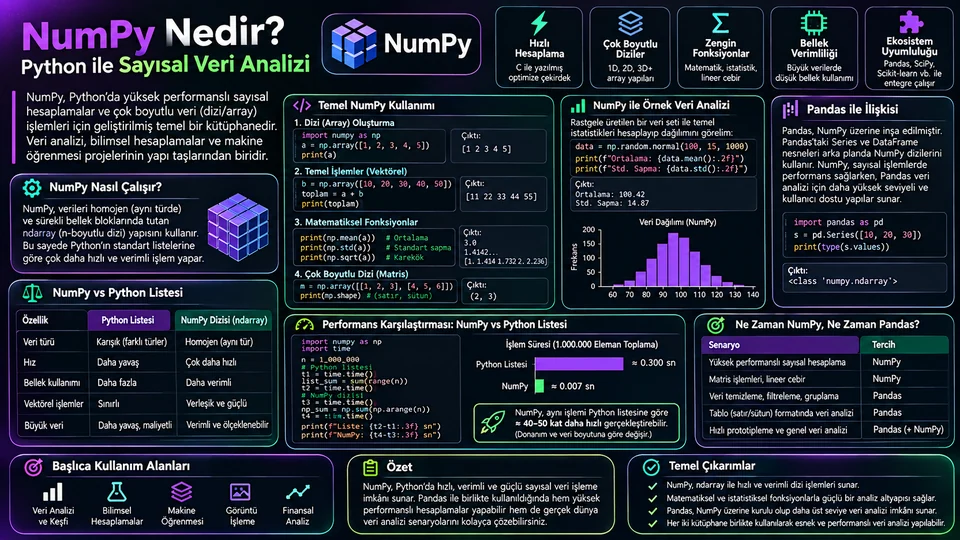
NumPy Nedir? Python ile Sayısal Veri Analizi
ndarray'in şekli, axis yönü ve broadcasting kuralları. NumPy'yi gerçekten kullanabilmek için bilmeniz gereken dört kavramı, en sık yapılan hatalarla birlikte örnek kodlar üzerinden anlatıyorum.
- Araçlar
NumPy nedir?
NumPy, Python'da sayısal hesaplamanın temel kütüphanesidir. Ana veri yapısı ndarray, aynı türden elemanları çok boyutlu bir ızgarada tutar. Listelerden farkı şu: bir NumPy dizisindeki bütün elemanlar aynı türdedir ve bellekte bitişik durur. Bu kısıt, karşılığında büyük bir avantaj verir — tüm diziye tek seferde matematiksel işlem uygulanabilir.
Bu yüzden NumPy yalnızca kendi başına kullanılan bir araç değil, bir altyapıdır. pandas, scikit-learn, SciPy, matplotlib ve daha pek çok kütüphane sayısal veriyi NumPy dizileri üzerinden alıp verir. Veri analisti olarak pandas'tan çıkmasanız bile, arka planda çalışan şeyin ne olduğunu bilmek hata ayıklarken işinize yarar.
ndarray ve dizinin üç özelliği
Bir diziyle çalışırken sürekli bakacağınız üç şey var: ndim (kaç eksen var), shape (her eksende kaç eleman var) ve dtype (elemanlar hangi türde). Bir hata aldığınızda ilk refleksiniz bu üçünü yazdırmak olsun; vakaların çoğu burada çözülür.
import numpy as np

puan = np.array([72, 85, 91, 68])
matris = np.array([[12, 15, 14],
                   [18, 17, 20]])

print(puan.ndim, puan.shape, puan.dtype)   # 1 (4,) int64
print(matris.ndim, matris.shape)          # 2 (2, 3)

print(np.zeros((2, 3)))      # sıfırlarla doldurulmuş
print(np.arange(0, 10, 2))   # [0 2 4 6 8] — adımlı
print(np.linspace(0, 1, 5))  # [0. 0.25 0.5 0.75 1.] — eşit aralıklı
shape değeri (2, 3) ise iki satır ve üç sütun demektir. arange ile linspace arasındaki farkı karıştırmak yaygın bir hatadır: ilki adım büyüklüğünü, ikincisi kaç değer isteyeceğinizi alır. Kayan noktalı adımlarda arange yuvarlama nedeniyle beklediğinizden bir eleman eksik veya fazla üretebilir; eşit aralıklı bir ızgara istiyorsanız linspace daha güvenlidir.
float64 yerine float32 seçmek belleği yarıya indirir ama hassasiyeti de düşürür. Türü bilinçli seçin, varsayılana güvenmeyin.İndeksleme, dilimleme ve maskeler
Tek boyutlu diziler Python listeleri gibi dilimlenir. Çok boyutlularda her ekseni virgülle ayırırsınız. Analizde en çok kullanacağınız biçim ise boole maske: bir koşul yazarsınız, dizi o koşulu sağlayan elemanları döndürür.
degerler = np.array([11, 24, 8, 31, 19])

print(degerler[1])              # 24
print(degerler[1:4])            # [24  8 31] — 4 hariç
print(degerler[degerler >= 18])  # [24 31 19]

olcum = np.array([[5.2, 7.1, 6.8],
                  [4.9, 8.3, 7.5]])

print(olcum[0, 1])            # 7.1 — ilk satır, ikinci sütun
print(olcum[:, 0])             # [5.2 4.9] — tüm satırların ilk sütunu
Burada çoğu insanın bir kez yandığı bir ayrıntı var: temel dilimleme çoğu zaman görünüm (view) döndürür, kopya değil. Yani dilimi değiştirdiğinizde kaynak dizi de değişir.
a = np.arange(6).reshape(2, 3)
b = a[:, 0]      # görünüm
b[0] = 99

print(a[0, 0])    # 99  → kaynak dizi de değişti

c = a[:, 0].copy()   # bağımsız kopya
c[0] = -1
print(a[0, 0])    # 99  → kaynak etkilenmedi
Bu davranış kasıtlıdır ve bellek tasarrufu sağlar. Ama bir fonksiyona dilim geçirip içeride değiştirdiğinizde çağıran tarafın verisini de bozarsınız. Değiştireceğiniz şey bağımsız olmalıysa .copy() yazın.
Eleman bazlı matematik ve ufunc'lar
Aynı şekle sahip iki dizide toplama, çıkarma ve çarpma eleman eleman yapılır. NumPy'nin evrensel fonksiyonları (ufunc) — sqrt, exp, log, sin — her elemana ayrı ayrı uygulanır.
a = np.array([2.0, 4.0, 8.0])
b = np.array([1.0, 3.0, 5.0])

print(a + b)          # [ 3.  7. 13.]
print(a * b)          # [ 2. 12. 40.]
print(a ** 2)         # [ 4. 16. 64.]
print(np.sqrt(a))
print(np.where(a > 3, "yüksek", "düşük"))
En sık karıştırılan nokta burada: NumPy'de * matris çarpımı değildir. Eleman bazlı çarpımdır. Lineer cebir çarpımı için @ operatörünü veya np.matmul'u kullanın.
A = np.array([[1, 2], [3, 4]])
B = np.array([[2, 0], [1, 2]])

print(A * B)   # [[2 0]
              #  [3 8]]  → eleman bazlı
print(A @ B)   # [[ 4  4]
              #  [10  8]] → matris çarpımı
İki sonuç da hata vermeden döner; yanlış olanı seçtiğinizde kod çalışmaya devam eder ve sessizce yanlış sayılar üretir. Bu yüzden lineer cebir yazarken hangisini istediğinizi bilinçli olarak seçin.
İstatistiksel özetler ve axis
sum, mean, median, std, min, max dizinin özetini verir. Çok boyutlu dizilerde kritik parametre axis'tir ve en çok burada hata yapılır. Şöyle düşünün: axis, ortadan kaldırılacak ekseni söyler. İki boyutlu bir tabloda axis=0 satırları toplar ve geriye sütun başına bir değer bırakır; axis=1 sütunları toplar ve satır başına bir değer bırakır.
notlar = np.array([[70, 82, 91],
                   [88, 76, 84],
                   [95, 90, 87]])

print(notlar.mean())         # 84.78 — tüm değerler
print(notlar.mean(axis=0))   # [84.33 82.67 87.33] — ders ortalamaları
print(notlar.mean(axis=1))   # [81. 82.67 90.67] — öğrenci ortalamaları
Hangisini istediğinizden emin değilseniz küçük bir örnekle test edin: 3×3'lük bir diziye axis=0 uyguladığınızda sonuç 3 elemanlı bir dizi olmalı ve o değerler sütunlara ait olmalı. Bunu bir kez doğruladıktan sonra büyük veride tereddüt etmezsiniz.
NaN varsa mean() sonucu da NaN olur. np.nanmean, np.nansum gibi fonksiyonlar eksikleri atlar — ama "eksik değeri yok saymak" her analizde doğru karar değildir. Önce eksikliğin neden olduğuna bakın.Broadcasting: farklı şekilleri birlikte kullanmak
Broadcasting, uyumlu şekillere sahip dizilerin, veriyi kopyalamadan birlikte işlenmesini sağlar. Kural şudur: şekiller sağdan sola karşılaştırılır; her konumda boyutlar ya eşit olmalı ya da biri 1 olmalıdır.
X = np.array([[10., 100.],
              [12., 130.],
              [14., 110.]])          # şekil (3, 2)

sutun_ort = X.mean(axis=0)                 # şekil (2,)
merkezli = X - sutun_ort                      # (3,2) - (2,) yayınlanır

print(merkezli.mean(axis=0))             # ~[0. 0.]
Burada (2,) şekilli dizi, sağdan hizalanarak (3, 2)'ye yayılır ve her satırdan aynı sütun ortalamaları çıkarılır. Satır bazında bir işlem isteseydiniz, X.mean(axis=1) sonucunu .reshape(-1, 1) ile sütun vektörüne çevirmeniz gerekirdi.
| Şekil A | Şekil B | Sonuç | Neden? |
|---|---|---|---|
| (3, 2) | (2,) | (3, 2) | Sağdan hizalanır: 2 = 2, eksik eksen 1 sayılır |
| (3, 2) | (3, 1) | (3, 2) | Son eksende 1 var, genişletilir |
| (3, 2) | (3,) | Hata | Son eksen 2 ile 3 uyuşmuyor |
| (4, 1) | (1, 5) | (4, 5) | İki yönde de genişler — dış çarpım etkisi |
Son satır önemli bir uyarı: farkında olmadan (4, 1) ile (1, 5) topladığınızda 20 elemanlı bir dizi üretirsiniz. Gerçek veride bu, beklediğinizden bin kat büyük bir ara dizi anlamına gelebilir. Hata aldığınızda ya da sonuç tuhafsa önce shape değerlerini yazdırın.
Performans gerçekten nereden geliyor?
NumPy'nin hızı iki şeyden gelir: veriler bellekte bitişik ve tek türde durur, işlemler de derlenmiş kodda döner. Python'un eleman başına nesne yükü ve döngü maliyeti ortadan kalkar.
olcum = np.array([12.5, 14.0, 9.5, 16.0])

# Döngülü: her eleman için Python seviyesinde iş
celsius = [(x - 32) * 5 / 9 for x in olcum]

# Vektörleştirilmiş: tek ifade, tüm dizi
celsius = (olcum - 32) * 5 / 9
Buna rağmen "NumPy her zaman daha hızlıdır" demek doğru olmaz. Birkaç yüz elemanlı dizilerde kurulum maliyeti baskın gelebilir. Ayrıca her ara işlem yeni bir dizi üretir; uzun bir zincir, farkında olmadan birkaç kopya oluşturur. Zaman kritikse ölçün — tahmin etmeyin.
%timeit sihirli komutudur. Kendi verinizle, gerçek boyutta ölçün; internetteki bir karşılaştırma sizin veri boyutunuzda geçerli olmayabilir.NumPy ve pandas: hangisi ne zaman?
pandas, etiketli satır ve sütunlarla tablo verisini yönetmek için tasarlanmıştır; sayısal işlemlerin önemli bir kısmında NumPy altyapısından yararlanır. Kabaca iş bölümü şudur: etiket, farklı sütun türleri, birleştirme, gruplama ve eksik değer yönetimi pandas'ın işidir; homojen sayısal diziler, matris işlemleri ve kütüphane girdileri NumPy'nin.
import pandas as pd

df = pd.DataFrame({
    "urun": ["A", "B", "C"],
    "fiyat": [10.0, 15.0, 12.0],
    "adet": [3, 2, 5],
})

df["ciro"] = df["fiyat"] * df["adet"]   # pandas tarafı

X = df[["fiyat", "adet"]].to_numpy()      # NumPy tarafı
print(X.mean(axis=0))
to_numpy() etiketleri taşımaz: sütun adları ve satır indeksi dizide yoktur. Bu yüzden sütun sırasını açıkça yazın — modele hangi sütunun hangi sırayla gittiğini sonradan hatırlamaya çalışmak, en sessiz hata kaynaklarından biridir. Ayrıca farklı türlerde sütunları birlikte dönüştürürseniz NumPy ortak bir tür seçer ve sayılar metne dönüşebilir.
Kontrol listesi
- Şekli yazdırın. Hata ayıklamaya
ndim,shapevedtypeile başlayın. - Matris çarpımında
@kullanın.*eleman bazlıdır ve sessizce yanlış sonuç verir. - axis yönünü küçük örnekle doğrulayın. 3×3 bir diziyle bir kez test etmek yeter.
- Broadcasting boyutlarını denetleyin. Beklenmedik büyüklükte ara dizi üretmediğinizden emin olun.
- Gerektiğinde
.copy()alın. Dilim çoğu zaman görünümdür, kopya değil. - NaN davranışını açıkça seçin.
nanmeankullanmak bir karardır, varsayılan değil. - Sütun sırasını sabitleyin.
to_numpy()sonrası etiket yoktur. - Performansı kendi verinizde ölçün. Küçük dizide vektörleştirme avantaj getirmeyebilir.
Sonuç
NumPy'yi öğrenmek, aslında dört kavramı öğrenmektir: ndarray'in şekli, eleman bazlı işlemler, axis yönü ve broadcasting kuralları. Bu dördünü oturttuğunuzda hem kodunuz kısalır hem de pandas, scikit-learn ve matplotlib'in neden böyle davrandığını anlarsınız.
Pratik yaklaşım şu: tabloyu pandas ile keşfedin, sayısal çekirdeği NumPy'ye bırakın, sonucu etiketli biçimde tabloya geri yazın. Arada bir şey ters gittiğinde de ilk bakacağınız yer belli — shape ve dtype.
What is NumPy?
NumPy is the foundational library for numerical computing in Python. Its core data structure, the ndarray, holds elements of a single type in a multi-dimensional grid. The difference from a list is this: every element in a NumPy array has the same type and they sit contiguously in memory. That constraint buys you something big in return — a mathematical operation can be applied to the whole array at once.
So NumPy is not only a tool you use directly, it is infrastructure. pandas, scikit-learn, SciPy, matplotlib and many others pass numerical data around as NumPy arrays. Even if you never leave pandas as an analyst, knowing what runs underneath helps when you are debugging.
ndarray and the three attributes
There are three things you will keep checking when working with arrays: ndim (how many axes), shape (how many elements along each axis) and dtype (what type the elements are). Make printing those three your first reflex when something breaks; most cases get solved right there.
import numpy as np

scores = np.array([72, 85, 91, 68])
matrix = np.array([[12, 15, 14],
                   [18, 17, 20]])

print(scores.ndim, scores.shape, scores.dtype)  # 1 (4,) int64
print(matrix.ndim, matrix.shape)                # 2 (2, 3)

print(np.zeros((2, 3)))      # filled with zeros
print(np.arange(0, 10, 2))   # [0 2 4 6 8] — by step
print(np.linspace(0, 1, 5))  # [0. 0.25 0.5 0.75 1.] — evenly spaced
A shape of (2, 3) means two rows and three columns. Mixing up arange and linspace is a common slip: the first takes a step size, the second takes how many values you want. With floating-point steps, arange can produce one element more or fewer than you expected because of rounding; if you want an evenly spaced grid, linspace is safer.
float32 over float64 halves the memory but also lowers precision. Pick the type deliberately rather than trusting the default.Indexing, slicing and masks
One-dimensional arrays slice like Python lists. In multi-dimensional arrays you separate each axis with a comma. The form you will use most in analysis is the boolean mask: you write a condition and the array returns the elements that satisfy it.
values = np.array([11, 24, 8, 31, 19])

print(values[1])             # 24
print(values[1:4])           # [24  8 31] — 4 excluded
print(values[values >= 18])   # [24 31 19]

readings = np.array([[5.2, 7.1, 6.8],
                     [4.9, 8.3, 7.5]])

print(readings[0, 1])        # 7.1 — first row, second column
print(readings[:, 0])         # [5.2 4.9] — first column of every row
There is a detail here that catches most people once: basic slicing usually returns a view, not a copy. Change the slice and the source array changes too.
a = np.arange(6).reshape(2, 3)
b = a[:, 0]      # a view
b[0] = 99

print(a[0, 0])    # 99  → the source array changed too

c = a[:, 0].copy()   # an independent copy
c[0] = -1
print(a[0, 0])    # 99  → the source is untouched
The behaviour is deliberate and saves memory. But pass a slice into a function and modify it in place, and you corrupt the caller's data as well. If what you modify needs to be independent, write .copy().
Element-wise maths and ufuncs
For two arrays of the same shape, addition, subtraction and multiplication happen element by element. NumPy's universal functions (ufuncs) — sqrt, exp, log, sin — are applied to each element separately.
a = np.array([2.0, 4.0, 8.0])
b = np.array([1.0, 3.0, 5.0])

print(a + b)          # [ 3.  7. 13.]
print(a * b)          # [ 2. 12. 40.]
print(a ** 2)         # [ 4. 16. 64.]
print(np.sqrt(a))
print(np.where(a > 3, "high", "low"))
Here is the most frequently confused point: in NumPy, * is not matrix multiplication. It is element-wise. For the linear-algebra product use the @ operator or np.matmul.
A = np.array([[1, 2], [3, 4]])
B = np.array([[2, 0], [1, 2]])

print(A * B)   # [[2 0]
              #  [3 8]]  → element-wise
print(A @ B)   # [[ 4  4]
              #  [10  8]] → matrix product
Both return without an error; pick the wrong one and your code keeps running while quietly producing wrong numbers. So when you write linear algebra, choose consciously.
Statistical summaries and axis
sum, mean, median, std, min and max summarise an array. For multi-dimensional arrays the critical parameter is axis, and that is where most mistakes happen. Think of it this way: axis names the axis to be collapsed. In a two-dimensional table, axis=0 collapses the rows and leaves one value per column; axis=1 collapses the columns and leaves one value per row.
grades = np.array([[70, 82, 91],
                   [88, 76, 84],
                   [95, 90, 87]])

print(grades.mean())         # 84.78 — all values
print(grades.mean(axis=0))   # [84.33 82.67 87.33] — per course
print(grades.mean(axis=1))   # [81. 82.67 90.67] — per student
If you are unsure which one you want, test it on a small example: applying axis=0 to a 3×3 array should give three values, and those values should belong to the columns. Verify it once and you will not hesitate on real data.
NaN, the result of mean() is NaN too. Functions like np.nanmean and np.nansum skip missing values — but "ignore the missing value" is not the right decision in every analysis. Look at why it is missing first.Broadcasting: working across shapes
Broadcasting lets arrays with compatible shapes be combined without copying data. The rule: shapes are compared right to left, and at each position the dimensions must either be equal or one of them must be 1.
X = np.array([[10., 100.],
              [12., 130.],
              [14., 110.]])          # shape (3, 2)

col_mean = X.mean(axis=0)                  # shape (2,)
centred = X - col_mean                        # (3,2) - (2,) broadcasts

print(centred.mean(axis=0))              # ~[0. 0.]
The (2,) array is aligned from the right, stretched to (3, 2), and the same column means are subtracted from every row. If you wanted a row-wise operation instead, you would reshape X.mean(axis=1) into a column vector with .reshape(-1, 1).
| Shape A | Shape B | Result | Why? |
|---|---|---|---|
| (3, 2) | (2,) | (3, 2) | Right-aligned: 2 = 2, the missing axis counts as 1 |
| (3, 2) | (3, 1) | (3, 2) | The last axis is 1, so it is stretched |
| (3, 2) | (3,) | Error | Last axis 2 does not match 3 |
| (4, 1) | (1, 5) | (4, 5) | Stretches both ways — an outer-product effect |
That last row is a real warning: add a (4, 1) to a (1, 5) by accident and you get a 20-element array. On real data that can mean an intermediate array a thousand times larger than you expected. When you hit an error, or the result looks odd, print the shapes first.
Where the performance actually comes from
NumPy's speed comes from two things: the data sits contiguously in memory in a single type, and the operations run in compiled code. Python's per-element object overhead and loop cost disappear.
readings = np.array([12.5, 14.0, 9.5, 16.0])

# Looped: Python-level work per element
celsius = [(x - 32) * 5 / 9 for x in readings]

# Vectorised: one expression, whole array
celsius = (readings - 32) * 5 / 9
Even so, "NumPy is always faster" is not true. On arrays of a few hundred elements, setup cost can dominate. Every intermediate operation also produces a new array, so a long chain quietly creates several copies. If timing matters, measure it — do not guess.
%timeit magic in Jupyter. Measure with your own data at its real size; a benchmark you read online may not hold at your scale.NumPy and pandas: which, when?
pandas is designed to manage tabular data with labelled rows and columns, and it leans on NumPy for a good share of its numerical work. The rough division of labour: labels, mixed column types, joins, grouping and missing-value handling belong to pandas; homogeneous numeric arrays, matrix operations and library inputs belong to NumPy.
import pandas as pd

df = pd.DataFrame({
    "product": ["A", "B", "C"],
    "price": [10.0, 15.0, 12.0],
    "quantity": [3, 2, 5],
})

df["revenue"] = df["price"] * df["quantity"]   # pandas side

X = df[["price", "quantity"]].to_numpy()        # NumPy side
print(X.mean(axis=0))
to_numpy() does not carry labels: column names and the row index are not in the array. So write the column order explicitly — trying to remember later which column went into the model in which position is one of the quietest sources of error. And if you convert columns of different types together, NumPy picks a common type and your numbers can turn into strings.
Checklist
- Print the shape. Start debugging with
ndim,shapeanddtype. - Use
@for matrix products.*is element-wise and fails silently. - Verify the axis direction on a small example. Testing once on a 3×3 array is enough.
- Check broadcasting dimensions. Make sure you are not creating an unexpectedly large intermediate.
- Take a
.copy()when you need one. A slice is usually a view, not a copy. - Decide NaN behaviour explicitly. Using
nanmeanis a choice, not a default. - Fix the column order. After
to_numpy()there are no labels left. - Measure performance on your own data. Vectorising may not pay off on small arrays.
Conclusion
Learning NumPy really means learning four concepts: the shape of an ndarray, element-wise operations, the direction of axis, and the broadcasting rules. Once those settle, your code gets shorter and you start to understand why pandas, scikit-learn and matplotlib behave the way they do.
The practical approach: explore the table with pandas, hand the numeric core to NumPy, write the result back into the table with labels. And when something goes wrong, you know where to look first — shape and dtype.