Sosyal Medyada Trend Analizi Nasıl Yapılır?
Hacim arttı demek yetmez. Paylaşım ile kullanıcı sayısını ayırmaktan hareketli ortalamanın ilk günlerine, medyanın neden ortalamadan önemli olduğundan veri kesintisini gerçek düşüşten ayırmaya kadar.
- Sosyal Medya
- Araçlar
Trend analizi neyi gösterir?
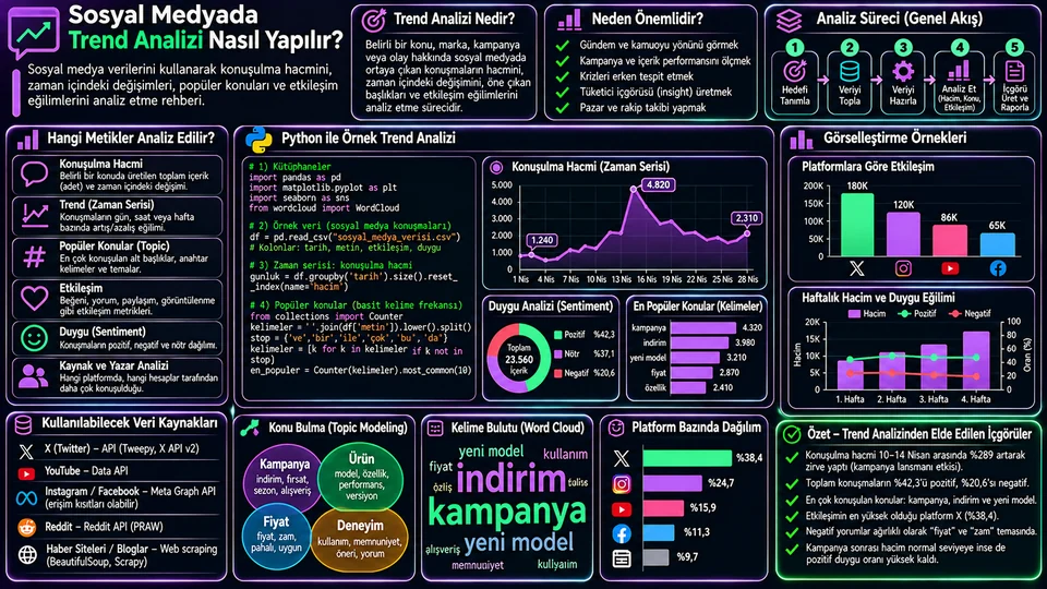
Sosyal medyada trend analizi, bir konu veya marka etrafındaki paylaşımların zaman içinde nasıl değiştiğini inceler. Amaç en çok konuşulan etiketi sıralamak değildir — asıl sorular şunlardır: artış ne zaman başladı, kalıcı mı yoksa tek günlük bir sıçrama mı, hangi alt konularla birlikte geldi, ve hacim artışı etkileşimde karşılık buldu mu?
Hacim
Gün veya saat başına paylaşım adedi. En temel ama tek başına en yanıltıcı gösterge.
Değişim
Önceki dönemle kıyas ve hareketli ortalama. Gürültüyü eğilimden ayırır.
Konu
Hashtag, anahtar sözcük veya sınıflandırılmış tema. "Neyi" konuştuklarını söyler.
Etkileşim
Beğeni, yanıt, paylaşım. Kaç kişinin umursadığını gösterir.
Analizi doğru tasarlamak
Veriyi çekmeden önce yapılacak işler, analizin kalitesini çekilen veriden daha çok belirler.
- Araştırma sorusunu yazın. "Marka hakkında ne konuşuluyor?" bir soru değildir. "Yeni ürün duyurusundan sonra marka konuşulma hacmi yükseldi mi, yükseldiyse ne kadar sürdü?" bir sorudur.
- Kapsamı sabitleyin. Tarih aralığı, dil, ülke, marka adının yazım varyantları, dâhil ve hariç tutulacak kelimeler. Marka adınız aynı zamanda genel bir kelimeyse (örneğin bir hayvan veya şehir adı), hariç tutma listesi analizin yarısıdır.
- Karşılaştırma tabanı seçin. Duyuru öncesi ve sonrası eşit uzunlukta dönemler, önceki yılın aynı haftası ya da benzer bir kontrol konusu. Taban olmadan "arttı" cümlesi anlamsızdır.
- Veri sözlüğü oluşturun. Hangi alan hangi platformdan geliyor, etkileşim nasıl tanımlanmış, saat dilimi ne?
- Sonucu elle doğrulayın. Rastgele 50 gönderi okuyun. Arama sorgunuz konu dışı içerik topluyorsa bunu ancak böyle fark edersiniz.
Veri yapısı ve ilk hazırlık
Analiz tablosunda en azından her paylaşım için zaman damgası ve metin bulunmalı. Etkileşim alanları platforma göre eksik veya farklı tanımlı olabilir.
| Alan | Açıklama | Not |
|---|---|---|
created_at | Paylaşım zamanı | Saat dilimini baştan standardize edin |
author_id | Paylaşan hesap | Benzersiz kullanıcı saymak için şart |
text | Metin içeriği | Kişisel veriyi gereksiz saklamayın |
likes, replies, shares | Etkileşim sayıları | Platform tanımıyla birlikte yorumlayın |
impressions | Gösterim sayısı | Her platformda bulunmaz |
import pandas as pd
import matplotlib.pyplot as plt
import seaborn as sns

df = pd.read_csv("sosyal_veri.csv")

df["created_at"] = pd.to_datetime(
    df["created_at"], utc=True, errors="coerce"
)
df = df.dropna(subset=["created_at"]).copy()

# Yerel saate çevir — saat bazlı analizde kritik
df["created_local"] = df["created_at"].dt.tz_convert("Europe/Istanbul")
df["gun"] = df["created_local"].dt.floor("D")

print("Kayıt:", len(df),
      "| Kullanıcı:", df["author_id"].nunique(),
      "| Aralık:", df["gun"].min(), "→", df["gun"].max())
Saat dilimi dönüşümünü atlamak, saat bazlı analizlerde sistematik hata üretir. UTC'de gece yarısı olan bir paylaşım, Türkiye saatiyle sabahın üçüdür — "en çok hangi saatte konuşuluyor?" sorusuna üç saat kaymış bir cevap verirsiniz.
Konuşulma hacmi ve değişim
En temel gösterge günlük paylaşım sayısıdır. Ham günlük çizgi dalgalıdır; hareketli ortalama bunu yumuşatır. İkisini birlikte çizin — sadece hareketli ortalamayı gösterirseniz ani sıçramayı gizlemiş olursunuz.
gunluk = (df.groupby("gun")
            .agg(paylasim=("text", "size"),
                 kullanici=("author_id", "nunique")))

gunluk["ort_7g"] = gunluk["paylasim"].rolling(7).mean()

sns.set_theme(style="whitegrid")
fig, ax = plt.subplots(figsize=(11, 5))
ax.plot(gunluk.index, gunluk["paylasim"], alpha=.4, label="Günlük paylaşım")
ax.plot(gunluk.index, gunluk["ort_7g"], linewidth=2.5, label="7 günlük ortalama")
ax.set(title="Günlük konuşulma hacmi", xlabel="Tarih", ylabel="Paylaşım")
ax.legend(); fig.tight_layout(); plt.show()rolling(7) varsayılan olarak ilk 6 günü NaN bırakır, çünkü henüz 7 gözlem yoktur. min_periods=1 eklerseniz boşluk kalmaz ama ilk günler 1-6 gözlemin ortalamasıdır — grafiğin başındaki o kısım diğerleriyle aynı şey değildir. Hangisini seçerseniz seçin, grafik notunda belirtin.Dönem değişimini hesaplamak
gunluk["onceki"] = gunluk["paylasim"].shift(1)

gunluk["degisim_pct"] = (
    (gunluk["paylasim"] - gunluk["onceki"])
    / gunluk["onceki"].replace(0, pd.NA) * 100
)

print(gunluk.tail(7).round(1))
Önceki dönem sıfırsa yüzde değişim tanımsızdır; sonsuz bir oran göstermeyin. Daha önemlisi: düşük hacimde yüzdeler yanıltıcıdır. 2 paylaşımdan 6'ya çıkmak %200 artıştır ama hiçbir şey ifade etmez. Her zaman mutlak sayıyı yüzdenin yanına yazın.
Popüler konular ve hashtag'ler
Etiket frekansı, neyin konuşulduğuna dair hızlı bir ipucu verir. Bir paylaşımda aynı etiket birden çok kez geçebileceği için, paylaşım başına her etiketi bir kez saymak daha doğru bir dağılım verir.
import re
from collections import Counter

def etiketleri_bul(metin):
    if not isinstance(metin, str):
        return set()
    # Paylaşım başına benzersiz etiket
    return set(re.findall(r"#([\wğüşöçıİĞÜŞÖÇ]+)", metin.lower()))

sayac = Counter(
    etiket for metin in df["text"]
    for etiket in etiketleri_bul(metin)
)

top = pd.Series(dict(sayac)).sort_values(ascending=False).head(10)

fig, ax = plt.subplots(figsize=(9, 5))
sns.barplot(x=top.values, y=["#" + t for t in top.index], ax=ax, color="#8b5cf6")
ax.set(title="En sık kullanılan 10 hashtag", xlabel="Paylaşım sayısı", ylabel="")
fig.tight_layout(); plt.show()
Türkçe metinlerde lower() kullanırken dikkat: Python'un lower() metodu yerel ayara duyarlı değildir, yani büyük "I" harfini noktasız "ı" yerine noktalı "i"ye çevirir. Marka adında büyük I varsa (örneğin "IGA"), bunu hesaba katın ve gerekirse manuel bir eşleme tablosu kullanın.
Etkileşim eğilimleri
Etkileşimi iki ayrı açıdan inceleyin: günlük toplam (toplam ilgi ne kadar) ve paylaşım başına ortalama (içerik ne kadar karşılık buluyor). İkisi aynı yönde hareket etmek zorunda değildir ve ayrıştıkları nokta genellikle en ilginç bulgudur.
etkilesim_sutunlari = ["likes", "replies", "shares"]
df[etkilesim_sutunlari] = df[etkilesim_sutunlari].fillna(0)
df["etkilesim"] = df[etkilesim_sutunlari].sum(axis=1)

gunluk_e = df.groupby("gun").agg(
    paylasim=("text", "size"),
    toplam=("etkilesim", "sum"),
    ortalama=("etkilesim", "mean"),
    medyan=("etkilesim", "median"),
)

# Gösterim verisi varsa ağırlıklı oran
if "impressions" in df.columns:
    gecerli = df["impressions"].gt(0)
    oran = (df.loc[gecerli, "etkilesim"].sum()
            / df.loc[gecerli, "impressions"].sum())
    print(f"Etkileşim/gösterim oranı: {oran:.2%}")
Tabloya medyanı da eklediğime dikkat edin. Tek bir viral paylaşım ortalamayı tamamen sürükler; medyan tipik paylaşımın ne kadar karşılık bulduğunu gösterir. Ortalama 450 ama medyan 3 ise, o günün etkileşimi tek bir gönderiden geliyor demektir — ve bu, raporun asıl haberidir.
Oran hesaplarken paydanın kapsamına dikkat edin: yalnızca gösterim verisi olan satırları kullandıysanız, oranı tüm veri için geçerliymiş gibi sunmayın. Platformlar etkileşimi farklı tanımlar; platformlar arası karşılaştırmada aynı ölçü gibi davranmayın.
Yorumlama: nereye dikkat etmeli?
| Gözlem | Aceleci yorum | Kontrol edilecek |
|---|---|---|
| Tek günlük zirve | "İlgi arttı" | Kaç benzersiz kullanıcı? Tek bir viral gönderi mi? |
| Kampanya sonrası artış | "Kampanya işe yaradı" | Aynı dönemde başka bir olay var mı? Kontrol grubu? |
| Hacim yüksek, etkileşim düşük | "Marka konuşuluyor" | Bot veya spam olabilir. Hesap yaşı ve tekrar oranına bakın. |
| Belirli saatte yoğunlaşma | "Kitlemiz o saatte aktif" | Saat dilimi doğru dönüştürüldü mü? |
| Ani düşüş | "İlgi azaldı" | Veri toplama kesintisi mi? API kotası doldu mu? |
Son satır özellikle önemli ve çok kaçırılır. Hacim grafiğinizde sıfıra inen bir gün, "o gün kimse konuşmadı" değil "o gün veri toplayamadık" olabilir. Bu ikisi grafikte tamamen aynı görünür. Bu yüzden veri toplama kapsamını ayrı bir seride izleyin: her gün kaç API çağrısı yapıldı, kaç kayıt geldi?
Tekrarlanabilir iş akışı
- Topla
- Temizle
- Sınıflandır
- Ölç
- Görselleştir
- Yorumla
- Raporla
- Topla: izinli kaynaktan, araştırma sorusuna uygun aralıkta; toplama kapsamını da kaydet.
- Temizle: zaman damgalarını standardize et, yinelenenleri ve bot şüphesi olan hesapları incele.
- Sınıflandır: konu sözlüğü oluştur, örnekleri elle doğrula.
- Ölç: hacim, benzersiz kullanıcı, dönem değişimi, hareketli ortalama, etkileşim.
- Görselleştir: zaman serisi için çizgi, konu sıralaması için yatay çubuk, saat-gün deseni için ısı haritası.
- Yorumla: değişimi olaylarla kıyasla, alternatif açıklamaları yaz.
- Raporla: kodu, filtreleri, tarih aralığını ve metrik formüllerini sakla; aynı akışla güncelle.
Sonuç
Sosyal medyada trend analizi, konuşmayı sayıya çevirmekten ibaret değildir. İyi bir analiz dört şeyi birlikte yapar: hacmi doğru tanımlar (paylaşım mı, kullanıcı mı?), zamansal değişimi gürültüden ayırır, konuları bağlamında okur ve etkileşimi adil bir paydayla ölçer.
Raporu yazarken şu beş şeyi eklemeyi alışkanlık hâline getirin: metrik tanımı, veri kapsamı, görsel, olası alternatif açıklamalar ve bilmediğiniz şeyler. Son madde en değerlisidir — "bu veri yalnızca Türkçe paylaşımları ve yalnızca X platformunu kapsıyor" cümlesi, grafiğin olduğundan fazla kesinlik izlenimi vermesini engeller.
What does trend analysis show?
Social media trend analysis examines how posts around a topic or brand change over time. The goal is not to rank the most-used hashtag — the real questions are: when did the rise begin, is it lasting or a one-day spike, which sub-topics came with it, and did the extra volume translate into engagement?
Volume
Posts per day or hour. The most basic indicator, and on its own the most misleading.
Change
Comparison with the previous period and a moving average. Separates noise from trend.
Topic
Hashtags, keywords or classified themes. Tells you what is being discussed.
Engagement
Likes, replies, shares. Shows how many people actually cared.
Designing the analysis properly
The work you do before pulling any data determines the quality of the analysis more than the data itself does.
- Write down the research question. "What are people saying about the brand?" is not a question. "Did brand conversation volume rise after the product announcement, and if so for how long?" is.
- Fix the scope. Date range, language, country, spelling variants of the brand name, included and excluded keywords. If your brand name is also an ordinary word (an animal or a city, say), the exclusion list is half the analysis.
- Choose a comparison baseline. Equal-length windows before and after the announcement, the same week last year, or a similar control topic. Without a baseline, the sentence "it went up" means nothing.
- Build a data dictionary. Which field comes from which platform, how is engagement defined, what is the time zone?
- Verify the result by hand. Read 50 random posts. That is the only way you will notice your search query is picking up off-topic content.
Data structure and first preparation
At minimum your analysis table needs a timestamp and the text for every post. Engagement fields may be missing or defined differently depending on the platform.
| Field | Description | Note |
|---|---|---|
created_at | Time of the post | Standardise the time zone up front |
author_id | The posting account | Essential for counting unique users |
text | Text content | Do not store personal data unnecessarily |
likes, replies, shares | Engagement counts | Interpret with the platform's definition |
impressions | Impression count | Not available on every platform |
import pandas as pd
import matplotlib.pyplot as plt
import seaborn as sns

df = pd.read_csv("social_data.csv")

df["created_at"] = pd.to_datetime(
    df["created_at"], utc=True, errors="coerce"
)
df = df.dropna(subset=["created_at"]).copy()

# Convert to local time — critical for hour-of-day analysis
df["created_local"] = df["created_at"].dt.tz_convert("Europe/Istanbul")
df["day"] = df["created_local"].dt.floor("D")

print("Records:", len(df),
      "| Users:", df["author_id"].nunique(),
      "| Range:", df["day"].min(), "→", df["day"].max())
Skipping the time zone conversion introduces a systematic error in hour-based analysis. A post at midnight UTC is three in the morning Turkish time — you would answer "what hour do people talk most?" with a three-hour shift.
Conversation volume and change
The most basic indicator is the daily post count. The raw daily line is jumpy; a moving average smooths it. Plot both — if you show only the moving average you have hidden the spike.
daily = (df.groupby("day")
           .agg(posts=("text", "size"),
                users=("author_id", "nunique")))

daily["avg_7d"] = daily["posts"].rolling(7).mean()

sns.set_theme(style="whitegrid")
fig, ax = plt.subplots(figsize=(11, 5))
ax.plot(daily.index, daily["posts"], alpha=.4, label="Daily posts")
ax.plot(daily.index, daily["avg_7d"], linewidth=2.5, label="7-day average")
ax.set(title="Daily conversation volume", xlabel="Date", ylabel="Posts")
ax.legend(); fig.tight_layout(); plt.show()rolling(7) leaves the first 6 days as NaN, because there are not yet 7 observations. Adding min_periods=1 removes the gap, but those first days are then the average of 1–6 observations — that part of the chart is not the same thing as the rest. Whichever you choose, say so in the chart note.Computing period change
daily["prev"] = daily["posts"].shift(1)

daily["change_pct"] = (
    (daily["posts"] - daily["prev"])
    / daily["prev"].replace(0, pd.NA) * 100
)

print(daily.tail(7).round(1))
If the previous period is zero, the percent change is undefined; do not display an infinite ratio. More importantly: at low volume, percentages mislead. Going from 2 posts to 6 is a 200% increase and means nothing. Always put the absolute number next to the percentage.
Popular topics and hashtags
Hashtag frequency gives a quick clue about what is being discussed. Because the same tag can appear several times in one post, counting each tag once per post gives a more faithful distribution.
import re
from collections import Counter

def find_tags(text):
    if not isinstance(text, str):
        return set()
    # Unique tags per post
    return set(re.findall(r"#([\wğüşöçıİĞÜŞÖÇ]+)", text.lower()))

counter = Counter(
    tag for text in df["text"]
    for tag in find_tags(text)
)

top = pd.Series(dict(counter)).sort_values(ascending=False).head(10)

fig, ax = plt.subplots(figsize=(9, 5))
sns.barplot(x=top.values, y=["#" + t for t in top.index], ax=ax, color="#8b5cf6")
ax.set(title="Ten most used hashtags", xlabel="Post count", ylabel="")
fig.tight_layout(); plt.show()
Be careful with lower() on Turkish text: Python's lower() is not locale-aware, so it maps a capital "I" to a dotted "i" rather than the dotless "ı". If your brand name contains a capital I, account for that and use a manual mapping where needed.
Engagement trends
Examine engagement from two angles: daily total (how much interest overall) and average per post (how well the content lands). The two do not have to move together, and where they diverge is usually the most interesting finding.
engagement_cols = ["likes", "replies", "shares"]
df[engagement_cols] = df[engagement_cols].fillna(0)
df["engagement"] = df[engagement_cols].sum(axis=1)

by_day = df.groupby("day").agg(
    posts=("text", "size"),
    total=("engagement", "sum"),
    mean=("engagement", "mean"),
    median=("engagement", "median"),
)

# Weighted rate where impression data exists
if "impressions" in df.columns:
    valid = df["impressions"].gt(0)
    rate = (df.loc[valid, "engagement"].sum()
            / df.loc[valid, "impressions"].sum())
    print(f"Engagement/impression rate: {rate:.2%}")
Note that I added the median to the table. One viral post drags the mean entirely; the median shows how a typical post performs. If the mean is 450 and the median is 3, that day's engagement came from a single post — and that is the actual headline of the report.
When computing rates, watch the scope of the denominator: if you used only rows that have impression data, do not present the rate as if it applied to the whole dataset. Platforms define engagement differently; do not treat it as the same measure across platforms.
Interpretation: what to watch for
| Observation | Hasty reading | What to check |
|---|---|---|
| A one-day peak | "Interest rose" | How many unique users? A single viral post? |
| Rise after a campaign | "The campaign worked" | Any other event in the same window? A control group? |
| High volume, low engagement | "The brand is being talked about" | Could be bots or spam. Check account age and repetition. |
| Concentration at one hour | "Our audience is active then" | Was the time zone converted correctly? |
| A sudden drop | "Interest fell" | A collection outage? Did the API quota run out? |
That last row matters especially and is missed often. A day that drops to zero on your volume chart may not be "nobody talked" but "we could not collect". The two look identical on a chart. So track collection coverage as its own series: how many API calls were made each day, how many records came back?
A repeatable workflow
- Collect
- Clean
- Classify
- Measure
- Visualise
- Interpret
- Report
- Collect: from a permitted source, over a window that fits the question; record the collection coverage too.
- Clean: standardise timestamps, examine duplicates and suspected bot accounts.
- Classify: build a topic dictionary and verify samples by hand.
- Measure: volume, unique users, period change, moving average, engagement.
- Visualise: a line for the time series, a horizontal bar for topic ranking, a heatmap for the hour-of-day pattern.
- Interpret: compare changes against events, write down the alternative explanations.
- Report: keep the code, the filters, the date range and the metric formulas; update through the same flow.
Conclusion
Social media trend analysis is more than turning conversation into numbers. A good analysis does four things at once: it defines volume precisely (posts or users?), separates temporal change from noise, reads topics in context, and measures engagement with a fair denominator.
When writing the report, make a habit of including five things: the metric definition, the data coverage, the chart, plausible alternative explanations, and what you do not know. The last is the most valuable — a sentence like "this data covers only Turkish-language posts and only one platform" keeps the chart from projecting more certainty than it has.